The Benchmarks¶

This section presents a very high-level overview of all the benchmark test suites I have considered and also an extremely high-level analysis of the results obtained with the different solvers across all benchmarks.

The conclusions on this section are quantitative enough to get a feeling about a specific solver performance, but given the amount of information condensed in a few tables/figures the analysis presented here has to be complemented by the suite-by-suite examination of the results.

One thing is definitely sure: the No Free Lunch Theorem strikes again (NFL).

In this page, the results in tables and pictures are presented by benchmark test suite in alphabetical order, although the order of the HTML web pages containing the description of the test suites is different: I have sorted them by their widespread usage in the optimization community or by the level of interest/novelty they inspired to me. So, for example, the first HTML page after this section contains the SciPy Extended benchmark test suite, followed by GKLS and then GlobOpt and so on.

Stopping Conditions and Tolerances¶

As mentioned in the main page, all the test functions on almost all benchmark suites have known global optimum values: in the few cases where the global optimum value is unknown (or I was unable to calculate it via analysis) their value has been estimated by enormous grid searches plus repeated minimizations. I then considered an algorithm to be successful if:

$\lvert F_{known \hspace{3pt} minimum} - F_{algorithm \hspace{3pt} minimum} \rvert \leq 10^{-6}$

All the other checks for tolerances - be those on relative change on the objective function from one iteration to the other, or too small variations in the variables in the function domain - have been disabled or mercilessly and brutally commented out in the code for each solver.

For example, for nlopt algorithms like CRS2 or DIRECT, a way to ignore other tolerances and only use the formula above may be:

 import nlopt

 algorithm = nlopt.GN_DIRECT_L

 problem = nlopt.opt(algorithm, N)
 problem.set_min_objective(objective_function)
 problem.set_lower_bounds(lb)
 problem.set_upper_bounds(ub)

 problem.set_stopval(fglob + tolf)
 problem.set_maxeval(maxfun)
 problem.set_ftol_abs(-1)
 problem.set_ftol_rel(-1)
 problem.set_xtol_abs(-1)
 problem.set_xtol_rel(-1)

High-Level Description of the Test Suites¶

This whole exercise is made up of 6,825 test problems divided across 16 different test suites: most of these problems are of low dimensionality (2 to 6 variables) with a few benchmarks extending to 9+ variables. With all the sensitivities performed during this exercise on those benchmarks, the overall grand total number of functions evaluations stands at 3,859,786,025 - close to 4 billion. Not bad.

Each test suite has a separate section in the next pages, describing in a bit more detail what I have managed to understand from the approach used to create the benchmark suite - which in many cases is not much, but I hope I will be able to give a general idea of the main characteristics of each test suite, with a bunch of cool-looking pictures too...

So, in order of implementation, these are the benchmark suites:

SciPy Extended: 235 multivariate problems (where the number of independent variables ranges from 2 to 17), again with multiple local/global minima.

I have added about 40 new functions to the standard SciPy benchmarks and fixed a few bugs in the existing benchmark models in the SciPy repository.
GKLS: 1,500 test functions, with dimensionality varying from 2 to 6, generated with the super famous GKLS Test Functions Generator. I have taken the original C code (available at http://netlib.org/toms/) and converted it to Python.
GlobOpt: 288 tough problems, with dimensionality varying from 2 to 5, created with another test function generator which I arbitrarily named “GlobOpt”: https://www.researchgate.net/publication/225566516_A_new_class_of_test_functions_for_global_optimization . The original code is in C++ and I have bridged it to Python using Cython.

Many thanks go to Professor Marco Locatelli for providing an updated copy of the C++ source code.
MMTFG: sort-of an acronym for “Multi-Modal Test Function with multiple Global minima”, this test suite implements the work of Jani Ronkkonen: https://www.researchgate.net/publication/220265526_A_Generator_for_Multimodal_Test_Functions_with_Multiple_Global_Optima . It contains 981 test problems with dimensionality varying from 2 to 4. The original code is in C and I have bridge it to Python using Cython.
GOTPY: a generator of benchmark functions using the Bocharov-Feldbaum “Method-Min”, containing 400 test problems with dimensionality varying from 2 to 5. I have taken the Python implementation from https://github.com/redb0/gotpy and improved it in terms of runtime.

Original paper from http://www.mathnet.ru/php/archive.phtml?wshow=paper&jrnid=at&paperid=11985&option_lang=eng .
Huygens: this benchmark suite is very different from the rest, as it uses a “fractal” approach to generate test functions. It is based on the work of Cara MacNish on Fractal Functions. The original code is in Java, and at the beginning I just converted it to Python: given it was slow as a turtle, I have re-implemented it in Fortran and wrapped it using f2py, then generating 600 2-dimensional test problems out of it.
LGMVG: not sure about the meaning of the acronym, but the implementation follows the “Max-Set of Gaussians Landscape Generator” described in http://boyuan.global-optimization.com/LGMVG/index.htm . Source code is given in Matlab, but it’s fairly easy to convert it to Python. This test suite contains 304 problems with dimensionality varying from 2 to 5.
NgLi: Stemming from the work of Chi-Kong Ng and Duan Li, this is a test problem generator for unconstrained optimization, but it’s fairly easy to assign bound constraints to it. The methodology is described in https://www.sciencedirect.com/science/article/pii/S0305054814001774 , while the Matlab source code can be found in http://www1.se.cuhk.edu.hk/~ckng/generator/ . I have used the Matlab script to generate 240 problems with dimensionality varying from 2 to 5 by outputting the generator parameters in text files, then used Python to create the objective functions based on those parameters and the benchmark methodology.
MPM2: Implementing the “Multiple Peaks Model 2”, there is a Python implementation at https://github.com/jakobbossek/smoof/blob/master/inst/mpm2.py . This is a test problem generator also used in the smoof library, I have taken the code almost as is and generated 480 benchmark functions with dimensionality varying from 2 to 5.
RandomFields: as described in https://www.researchgate.net/publication/301940420_Global_optimization_test_problems_based_on_random_field_composition , it generates benchmark functions by “smoothing” one or more multidimensional discrete random fields and composing them. No source code is given, but the implementation is fairly straightforward from the article itself.
NIST: not exactly the realm of Global Optimization solvers, but the NIST StRD dataset can be used to generate a single objective function as “sum of squares”. I have used the NIST dataset as implemented in lmfit, thus creating 27 test problems with dimensionality ranging from 2 to 9.
GlobalLib: Arnold Neumaier maintains a suite of test problems termed “COCONUT Benchmark” and Sahinidis has converted the GlobalLib and PricentonLib AMPL/GAMS dataset into C/Fortran code (http://archimedes.cheme.cmu.edu/?q=dfocomp ). I have used a simple C parser to convert the benchmarks from C to Python.

The global minima are taken from Sahinidis or from Neumaier or refined using the NEOS server when the accuracy of the reported minima is too low. The suite contains 181 test functions with dimensionality varying between 2 and 9.
CVMG: another “landscape generator”, I had to dig it out using the Wayback Machine at http://web.archive.org/web/20100612044104/https://www.cs.uwyo.edu/~wspears/multi.kennedy.html , the acronym stands for “Continuous Valued Multimodality Generator”. Source code is in C++ but it’s fairly easy to port it to Python. In addition to the original implementation (that uses the Sigmoid as a softmax/transformation function) I have added a few others to create varied landscapes. 360 test problems have been generated, with dimensionality ranging from 2 to 5.
NLSE: again, not really the realm of Global optimization solvers, but Nonlinear Systems of Equations can be transformed to single objective functions to optimize. I have drawn from many different sources (Publications, ALIAS/COPRIN and many others) to create 44 systems of nonlinear equations with dimensionality ranging from 2 to 8.
Schoen: based on the early work of Fabio Schoen and his short note on a simple but interesting idea on a test function generator, I have taken the C code in the note and converted it into Python, thus creating 285 benchmark functions with dimensionality ranging from 2 to 6.

Many thanks go to Professor Fabio Schoen for providing an updated copy of the source code and for the email communications.
Robust: the last benchmark test suite for this exercise, it is actually composed of 5 different kind-of analytical test function generators, containing deceptive, multimodal, flat functions depending on the settings. Matlab source code is available at http://www.alimirjalili.com/RO.html , I simply converted it to Python and created 420 benchmark functions with dimensionality ranging from 2 to 6.

As a high-level summary, Table 0.1 below reports for each test suite the number of problems as a function of dimensionality, together with their totals.

**Table 0.1**: Dimensionality of the test functions for all the benchmark suites
Test Suite	N = 2	N = 3	N = 4	N = 5	N = 6+	Total
CVMG	90	90	90	90	0	360
GKLS	300	300	300	300	300	1,500
GlobalLib	76	23	26	9	47	181
GlobOpt	72	72	72	72	0	288
GOTPY	100	100	100	100	0	400
Huygens	600	0	0	0	0	600
LGMVG	76	76	76	76	0	304
MMTFG	312	330	339	0	0	981
MPM2	120	120	120	120	0	480
NgLi	60	60	60	60	0	240
NIST	6	7	3	2	9	27
NLSE	15	15	3	1	10	44
RandomFields	120	120	120	120	0	480
Robust	84	84	84	84	84	420
Schoen	57	57	57	57	57	285
SciPy Extended	193	13	13	6	10	235
Total	2,281	1,467	1,463	1,097	517	6,825

For pretty much all the test suites the value of the objective function at the global optimum (or optima) is known, and for many of those also the position of the global optimum (or optima) is also known. Since I only care about the value of the objective function at the global optimum (or optima), it didn’t bother me that some test suites didn’t have a way to know the position of the global optimum (or optima) in the search space.

Table 0.2 gives an indication of whether, for each benchmark suite, the optimal value of the objective function (FOPT) and the position(s) of the global optima (XOPT) in the search space is known beforehand. This is my analysis and it may easily be that I have missed a few technical detail by classifying a test suite in a way or another, i.e. maybe the position/value of the optima is known but I have failed to recognize/derive it.

In addition, Table 0.2 gives an indication of the “hardness” of a benchmark test suite, based on my results on applying all the optimizers under consideration with a given budget of number of function evaluations, and specifically a maximum of $NF = 2,000$ . The criteria for this classification are completely arbitrary, but I chose them to be:

Maximum allowed number of functions evaluations $NF = 2,000$
Conditions for the classification:

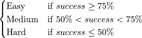
$\begin{cases} \textrm{Easy} & \textrm{if } success \geq 75 \% \\ \textrm{Medium} & \textrm{if } 50 \% < success < 75 \% \\ \textrm{Hard} & \textrm{if } success \leq 50 \% \\ \end{cases}$

The details are summarized in Table 0.2.

**Table 0.2**: Global optimum value and position assessment
Test Suite	F_opt Known	X_opt Known	Difficulty
CVMG	Yes	No	Medium
GKLS	Yes	Yes	Hard
GlobalLib	Yes	Yes	Easy
GlobOpt	Yes	No	Hard
GOTPY	Yes	Yes	Hard
Huygens	No	No	Medium
LGMVG	Yes	No	Easy
MMTFG	Yes	Yes	Easy
MPM2	Yes	Yes	Medium
NgLi	Yes	Yes	Easy
NIST	Yes	Yes	Medium
NLSE	Yes	Yes	Easy
RandomFields	No	No	Hard
Robust	Yes	Yes	Medium
Schoen	Yes	Yes	Easy
SciPy Extended	Yes	Yes	Easy

Aggregated, High-Level Results¶

This section provides some very high-level results stemming from the application of all nonlinear solvers to all the benchmark test suites. It is by no means a complete analysis but it does offer an insight on the various solvers performances, both in general, as a function of the dimensionality of the problem and as a function of the type of benchmark. Some test suites are much harder than others, and I have also tried to categorize the benchmark suites in terms of their “difficulty”, if that even makes sense.

I am going to present results in table and graphs, normally side-by-side or one after the other. I prefer the visuals, but I appreciate that quite a few people want to see the raw numbers. Since the amount of results available is kind of humongous, I have decided to present the high-level results for all solvers at two cutoffs in terms of function evaluations limits, and specifically $NF = 2,000$ and $NF = 10,000$ maximum evaluations.

General Results¶

Now, stopping the chit chat, Table 0.3 and Figure 0.1 below show the overall high-level results in terms of percentage of problems solved for each Global Optimization solver and each benchmark suite, at a 2,000 limit on function evaluations:

**Table 0.3**: Percentage of problems solved, per solver and benchmark suite at $NF = 2,000$
Test Suite	AMPGO	BasinHopping	BiteOpt	CMA-ES	CRS2	DE	DIRECT	DualAnnealing	LeapFrog	MCS	PSWARM	SCE	SHGO	Best Solver
CVMG	53.9%	55.0%	47.2%	50.8%	40.6%	48.3%	55.6%	54.2%	42.5%	56.4%	41.9%	50.6%	54.7%	MCS
GKLS	14.1%	15.5%	18.6%	7.1%	12.1%	13.7%	21.3%	24.0%	7.5%	28.5%	9.9%	12.1%	23.3%	MCS
GlobalLib	60.8%	53.0%	72.4%	43.1%	43.6%	39.8%	45.9%	59.7%	49.2%	80.7%	19.3%	56.4%	60.2%	MCS
GlobOpt	1.4%	10.4%	6.2%	0.3%	13.9%	4.5%	3.8%	5.6%	1.4%	6.9%	0.0%	0.3%	0.7%	CRS2
GOTPY	7.5%	3.2%	11.8%	3.0%	9.2%	6.2%	23.0%	8.8%	6.5%	17.5%	4.2%	7.8%	18.0%	DIRECT
Huygens	13.0%	2.0%	22.5%	8.0%	22.7%	36.5%	67.0%	2.8%	6.2%	11.5%	1.8%	14.5%	3.0%	DIRECT
LGMVG	46.4%	13.2%	43.8%	28.3%	50.7%	42.1%	65.8%	75.3%	32.6%	70.1%	20.4%	48.4%	77.6%	SHGO
MMTFG	60.2%	72.1%	72.3%	52.2%	49.8%	32.9%	59.4%	67.0%	43.9%	77.1%	19.6%	24.6%	69.2%	MCS
MPM2	36.0%	68.1%	35.0%	39.6%	35.0%	32.9%	59.8%	50.6%	23.8%	65.6%	21.2%	40.8%	65.2%	BasinHopping
NgLi	59.6%	32.5%	51.7%	56.2%	61.7%	43.3%	59.6%	68.8%	42.9%	86.7%	2.5%	77.9%	75.8%	MCS
NIST	33.3%	11.1%	48.1%	14.8%	25.9%	7.4%	3.7%	11.1%	18.5%	63.0%	0.0%	29.6%	7.4%	MCS
NLSE	63.6%	63.6%	75.0%	52.3%	38.6%	45.5%	47.7%	56.8%	54.5%	79.5%	27.3%	61.4%	65.9%	MCS
RandomFields	10.6%	19.4%	24.8%	9.2%	13.1%	19.8%	34.4%	34.2%	8.3%	29.4%	14.4%	17.1%	34.0%	DIRECT
Robust	52.1%	36.2%	62.4%	33.6%	40.5%	27.9%	45.7%	51.4%	22.9%	45.5%	28.1%	23.1%	36.4%	BiteOpt
Schoen	53.3%	90.2%	70.5%	71.2%	67.4%	52.3%	75.4%	85.6%	52.6%	91.2%	58.2%	68.4%	95.4%	SHGO
SciPy Extended	69.5%	64.7%	83.4%	58.8%	73.4%	75.4%	72.5%	72.4%	61.8%	81.9%	21.2%	71.2%	69.7%	BiteOpt
Weighted Average	39.1%	41.0%	46.1%	33.7%	37.8%	33.3%	51.8%	46.6%	28.4%	53.2%	18.6%	32.8%	48.6%	MCS

Figure 0.1 shows some sort of “heatmap”: the greener the color of a cell is, the better the performance of a specific solver is on the corresponding benchmarks. I have highlighted the “best” solver for each test suite in the picture with black square.

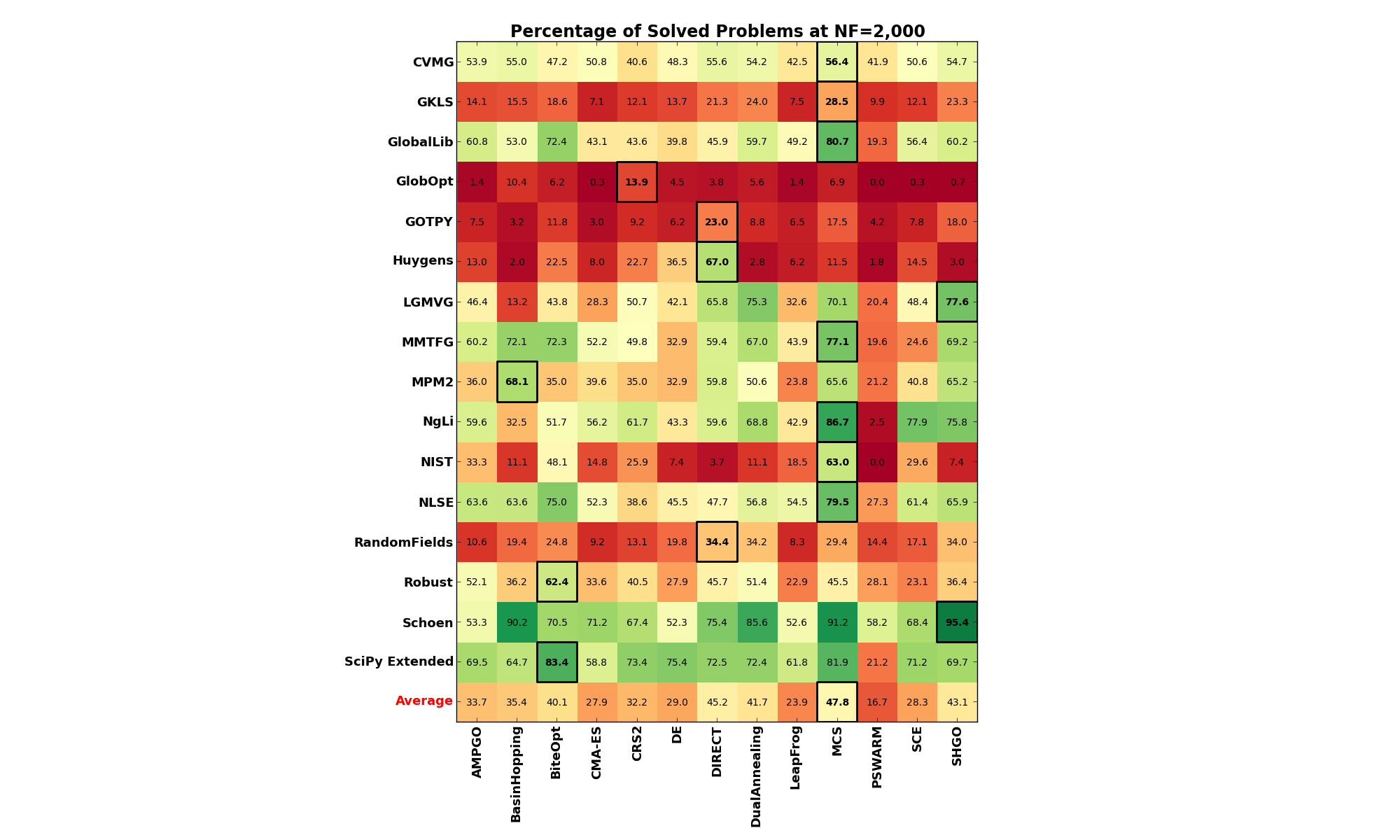
Percentage of problems solved, per solver and benchmark suite at :math:`NF = 2,000`

Figure 0.1: Percentage of problems solved, per solver and benchmark suite at $NF = 2,000$

Similarly, looking at problems solved for each Global Optimization solver and each benchmark suite, at a 10,000 limit on function evaluations (which is the maximum I have put in any benchmark test suite in this exercise):

**Table 0.4**: Percentage of problems solved, per solver and benchmark suite at $NF = 10,000$
Test Suite	AMPGO	BasinHopping	BiteOpt	CMA-ES	CRS2	DE	DIRECT	DualAnnealing	LeapFrog	MCS	PSWARM	SCE	SHGO	Best Solver
CVMG	58.3%	55.8%	49.2%	53.3%	40.6%	53.1%	56.1%	54.7%	42.5%	56.9%	48.9%	53.6%	56.1%	AMPGO
GKLS	26.6%	19.4%	22.8%	12.5%	13.7%	19.4%	28.6%	30.1%	7.5%	39.3%	19.5%	13.8%	29.5%	MCS
GlobalLib	71.8%	53.6%	79.0%	54.1%	67.4%	65.2%	48.6%	63.0%	54.7%	85.1%	44.8%	66.3%	61.9%	MCS
GlobOpt	5.9%	20.8%	10.8%	3.1%	18.4%	10.8%	10.4%	7.3%	1.4%	24.0%	7.3%	3.8%	3.8%	MCS
GOTPY	25.5%	5.0%	14.8%	6.8%	14.2%	14.2%	26.8%	10.5%	6.5%	43.5%	10.8%	10.0%	26.5%	MCS
Huygens	40.2%	4.5%	34.0%	22.3%	23.2%	36.8%	74.7%	9.0%	6.2%	27.7%	37.5%	35.8%	6.0%	DIRECT
LGMVG	73.0%	11.8%	49.7%	33.2%	57.6%	69.1%	73.7%	79.6%	32.6%	86.2%	57.9%	53.6%	95.1%	SHGO
MMTFG	75.8%	77.7%	78.9%	66.8%	61.1%	72.0%	64.4%	71.3%	43.9%	85.5%	67.7%	35.5%	78.7%	MCS
MPM2	59.2%	88.3%	39.0%	52.3%	37.1%	47.1%	68.8%	57.3%	23.8%	87.1%	47.1%	43.1%	80.0%	BasinHopping
NgLi	85.4%	33.3%	54.6%	82.1%	79.2%	82.5%	76.2%	72.9%	42.9%	96.2%	75.4%	79.6%	84.6%	MCS
NIST	51.9%	14.8%	70.4%	44.4%	70.4%	40.7%	3.7%	14.8%	22.2%	74.1%	7.4%	37.0%	7.4%	MCS
NLSE	75.0%	68.2%	90.9%	59.1%	52.3%	65.9%	52.3%	61.4%	65.9%	95.5%	54.5%	68.2%	65.9%	MCS
RandomFields	27.5%	28.5%	31.0%	16.2%	14.0%	34.0%	44.0%	41.5%	8.3%	49.4%	24.2%	26.7%	58.1%	SHGO
Robust	76.0%	41.7%	73.1%	58.1%	51.4%	59.0%	49.0%	64.8%	23.8%	59.5%	51.2%	31.2%	44.3%	AMPGO
Schoen	90.5%	95.1%	74.4%	78.9%	69.8%	74.4%	83.5%	87.7%	52.6%	96.8%	71.9%	69.5%	96.1%	MCS
SciPy Extended	80.7%	69.3%	89.8%	61.8%	79.8%	84.3%	77.9%	77.2%	62.7%	88.7%	75.9%	80.0%	77.1%	BiteOpt
Weighted Average	58.1%	46.6%	52.4%	44.9%	44.4%	52.8%	58.2%	51.6%	28.8%	66.6%	47.5%	40.7%	57.5%	MCS

And the corresponding image in Figure 0.2:

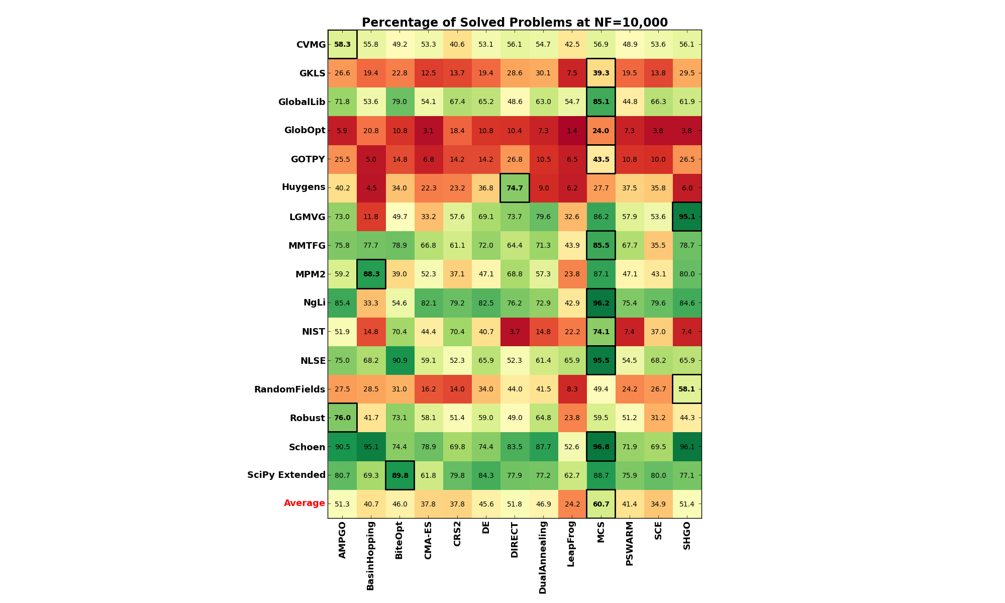
Percentage of problems solved, per solver and benchmark suite at :math:`NF = 10,000`

Figure 0.2: Percentage of problems solved, per solver and benchmark suite at $NF = 10,000$

There are some interesting conclusions to be drawn already: considering the test suites only for the moment, irrespective of the budget of function evaluations available, there seems to be very tough benchmark problems. The ones that stand out the most are GlobOpt, GOTPY, GKLS and Huygens. Even at very high limit on number of function evaluations, none of the solvers manages to solve more than 50% of the toughest three above.

Secondly, from the solvers point of view, it seems like MCS is doing quite a good job overall, followed by SHGO, DIRECT and BiteOpt. For a moderate budget (at $NF = 2,000$ ), MCS is the best solver for 8 of the 16 benchmark suites. At the maximum level of $NF = 10,000$ , MCS is the best solver for 10 of the 16 benchmark suites.

However, in order to draw any meaningful, very high-level conclusion on the solvers performances we have to deepen our analysis and consider the problem dimensionality and the variations in budget in terms of maximum number of functions evaluations allowed.

Dimensionality Effects¶

In this respect, we can first consider what fraction of problems each solver solved as a function of the benchmark dimensionality, and this is what the following two figures are showing (the first one at $NF = 2,000$ and the second one at $NF = 10,000$ ).

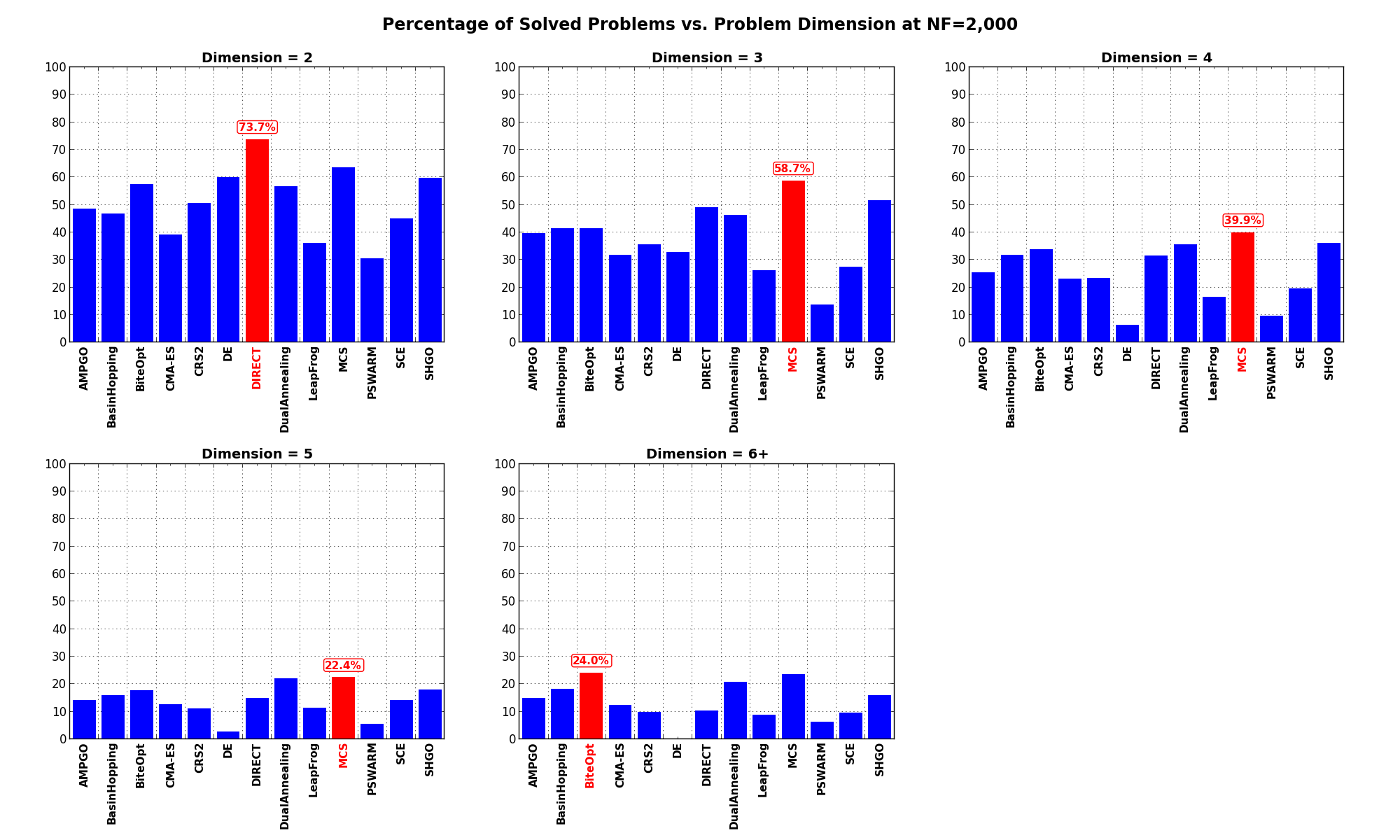
Figure 0.3: Percentage of problems solved as a function of problem dimension, per solver at $NF = 2,000$

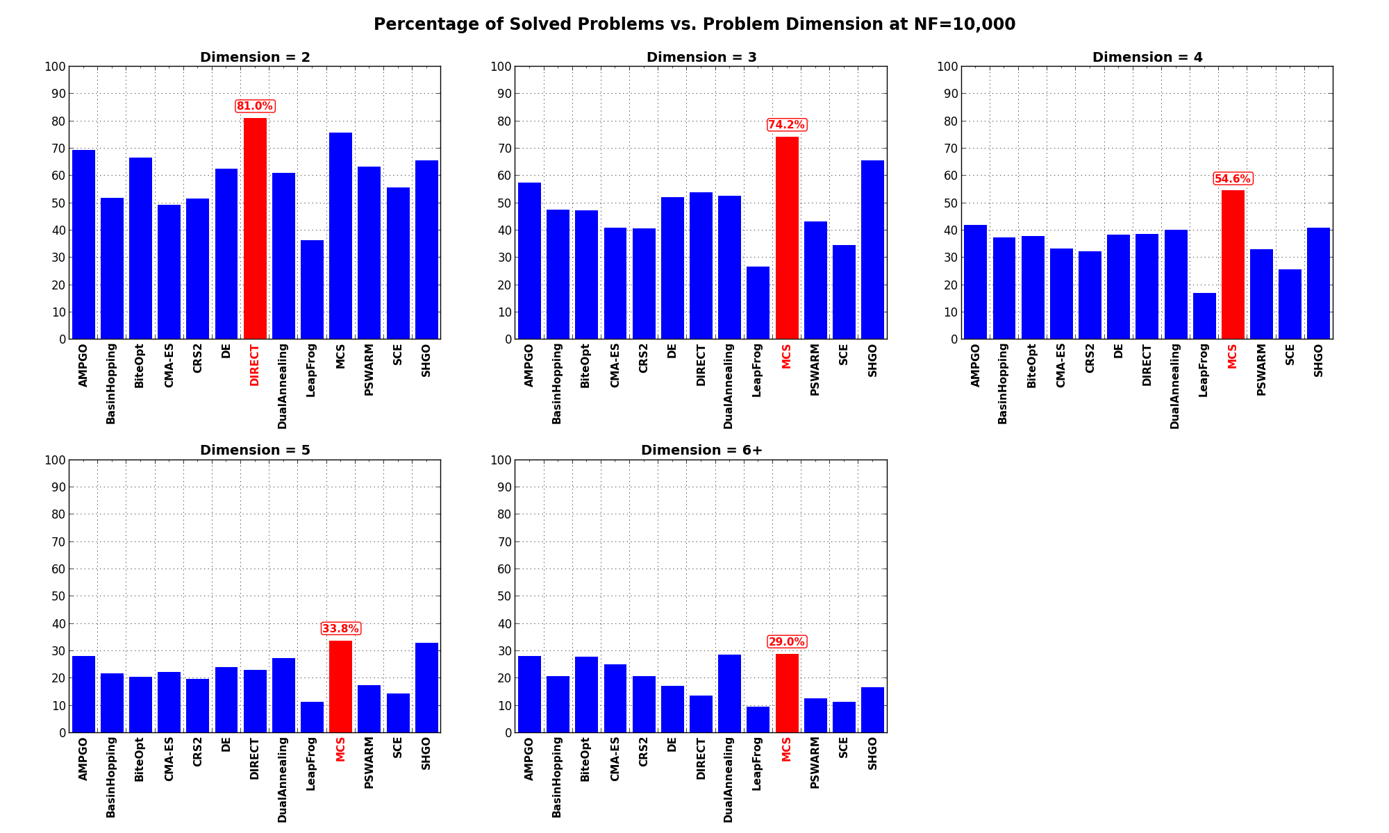
Figure 0.4: Percentage of problems solved as a function of problem dimension, per solver at $NF = 10,000$

What is interesting to see from these graphs is that MCS is always a very good contender, irrespective of the problem dimensionality, followed by SHGO, DualAnnealing and DIRECT, although the results for DIRECT are heavily skewed due to the good performances it has on the Huygens benchmark, which is composed exclusively by 2D functions (and very many of them, 600).

Expensive Objective Functions¶

If we consider, for a moment, a relatively tight budget in terms of available number of function evaluations, we could draw a potential conclusion on which solvers are the most effective when resources are scarce. Figure 0.5 shows exactly that, by displaying the percentage of problems solved when the budget is relatively limited ( $200 \leq NF \leq 500$ ).

Percentage of problems solved, per solver, at limited budget

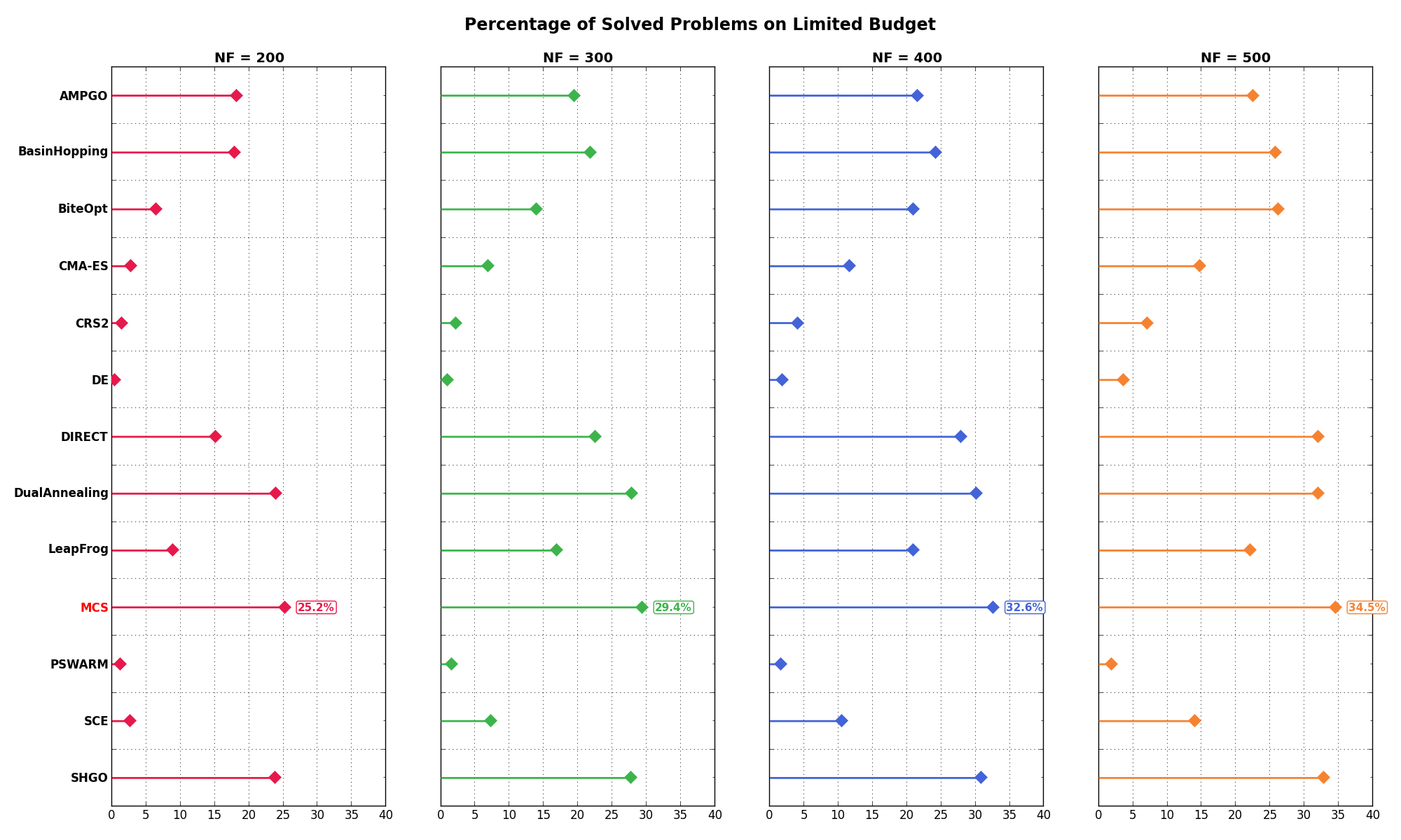
Figure 0.5: Percentage of problems solved for low budget function evaluations

There are two main high-level conclusions we can draw from Figure 0.5:

MCS appears to be the winner in this case too, even though it is by a very narrow margin.
The SciPy global solvers SHGO and DualAnnealing are among the best when the number of functions evaluations is limited - this is relatively common in real-life problems where the objective function may take several hours to compute.
AMPGO is unfortunately not as powerful anymore - this new set of benchmarks is much harder than my original tests in 2013.
Other solvers - such as BiteOpt, BasinHopping and AMPGO begin to catch up with the leaders only when the budget expands reasonably (i.e., $NF = 500$ ).

Simulation Time¶

While I don’t generally care about the performances of an optimization algorithm in terms of elapsed time, for this set of benchmarks I actually recorded the elapsed time for each solver - and specifically the average time spent by each solver in its own internal meanderings between each function evaluation.

Of course, each benchmark test suite is written in its own language - whether Python, C or Fortran - so the time spent evaluating a test function greatly vary between benchmarks but it is the same for all solvers for any specific test suite. In that sense, we can attempt some sort of “CPU” timings to see what are the fastest or slowest solvers in terms of time spent per function evaluation.

In Table 0.5 you can see the performances in terms of CPU time for each solver and each benchmark.

**Table 0.5**: Time spent per function evaluation in ms, per solver and benchmark suite at $NF = 2,000$
Test Suite	AMPGO	BasinHopping	BiteOpt	CMA-ES	CRS2	DE	DIRECT	DualAnnealing	LeapFrog	MCS	PSWARM	SCE	SHGO	Slowest Solver
CVMG	0.066	0.054	0.094	0.219	0.039	0.099	0.041	0.085	0.079	0.825	0.071	0.163	0.565	MCS
GKLS	0.067	0.050	0.094	0.152	0.050	0.096	0.051	0.084	0.085	1.098	0.046	0.166	1.023	MCS
GlobalLib	0.095	0.097	0.125	0.301	0.078	0.129	0.079	0.111	0.113	0.416	0.103	0.197	1.711	SHGO
GlobOpt	0.030	0.014	0.055	0.168	0.004	0.063	0.004	0.055	0.040	0.308	0.031	0.107	0.577	SHGO
GOTPY	0.072	0.062	0.109	0.215	0.054	0.115	0.056	0.093	0.094	0.364	0.082	0.171	0.273	MCS
Huygens	0.080	0.059	0.090	0.205	0.044	0.105	0.047	0.092	0.072	0.288	0.072	0.130	0.189	MCS
LGMVG	0.061	0.058	0.096	0.198	0.043	0.105	0.045	0.087	0.085	0.483	0.072	0.162	0.449	MCS
MMTFG	0.028	0.018	0.050	0.233	0.005	0.061	0.005	0.044	0.036	0.278	0.032	0.102	0.223	MCS
MPM2	0.434	0.415	0.458	0.580	0.403	0.467	0.405	0.451	0.442	0.828	0.440	0.531	0.764	MCS
NgLi	0.019	0.015	0.052	0.177	0.004	0.059	0.005	0.039	0.040	0.399	0.020	0.129	0.390	MCS
NIST	0.043	0.034	0.079	0.291	0.027	0.087	0.029	0.066	0.069	0.316	0.056	0.166	1.404	SHGO
NLSE	0.046	0.045	0.080	0.327	0.025	0.085	0.028	0.057	0.065	0.301	0.058	0.156	1.772	SHGO
RandomFields	1.302	1.293	1.317	1.583	1.256	1.342	1.255	1.328	1.291	1.636	1.284	1.360	1.854	SHGO
Robust	0.056	0.042	0.091	0.204	0.031	0.094	0.032	0.079	0.075	0.564	0.062	0.148	0.954	SHGO
Schoen	0.060	0.050	0.096	0.237	0.035	0.105	0.035	0.067	0.078	0.585	0.070	0.183	0.389	MCS
SciPy Extended	0.061	0.055	0.084	0.248	0.040	0.096	0.041	0.075	0.071	0.349	0.068	0.134	0.236	MCS
Weighted Average	0.171	0.159	0.197	0.326	0.147	0.205	0.148	0.189	0.183	0.679	0.169	0.259	0.707	SHGO

The table reflects exactly my feelings while I was running the different benchmark test suites. Test suites written in Python (and especially the ones re-coded by me) such as GKLS, RandomFields and MPM2 are not particularly performant. Other test suites, either originally coded in C and wrapped by in with Cython or the ones I have translated to Fortran - such as MMTFG and GlobOpt, are relatively fast overall.

The table also perfectly represent me impatiently waiting for MCS and SHGO to finish their optimizations, especially when varying the maximum number of function evaluations allowed from 100 to 10,000... it took forever for those two solvers to finish, and the higher the dimensionality the worse the problem becomes.

This can actually be seen in Figure 0.6, which shows the average CPU time spent by each solver per function evaluation as a function of the problem dimension in the GKLS benchmark. Pretty much all the other solvers are stable around a relatively low runtime (which of course depends on how busy my machine was - those numbers are also influenced by the fact that the benchmarks are run in parallel, with one CPU core per solver), except for MCS and SHGO.

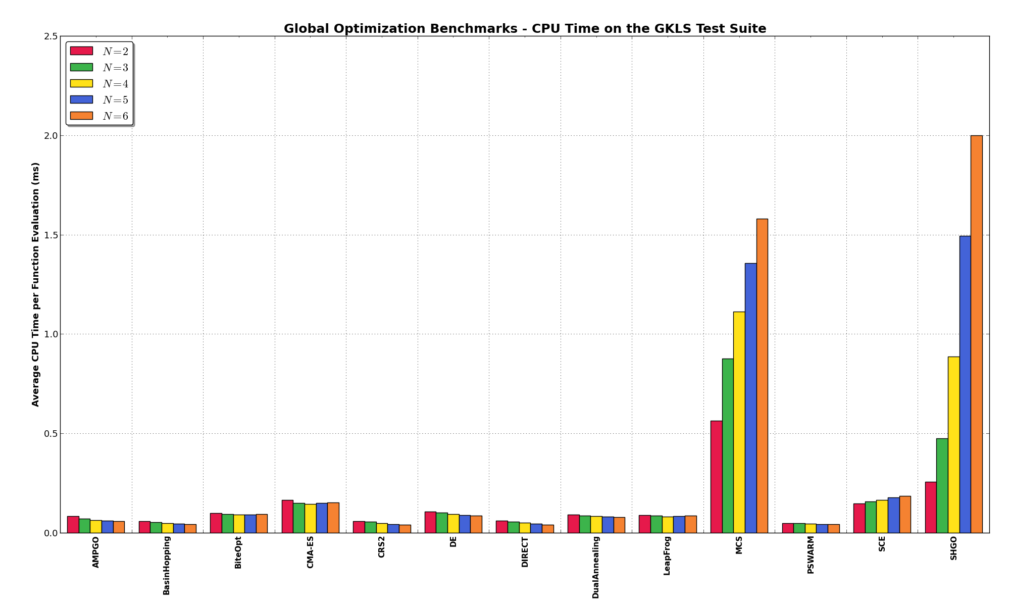
Figure 0.6: CPU runtime, per solver, for the GKLS test suite as a function of problem dimension

This behaviour is somehow to be expected, SHGO is explicitely targeted to low-dimensional problems, as explicitely stated in the “Notes”” section of https://docs.scipy.org/doc/scipy/reference/generated/scipy.optimize.shgo.html and MCS represents my translation (pretty much line by line) of an already inefficient Matlab code into a language even less efficient, Python.

Solvers - Example¶

To illustrate and contrast the search strategies that are employed by different algorithms, Figure 0.7 shows how the different solvers progress for the objective function SixHumpCamel. This two-dimensional test problem, referred to as the “six-hump camel back function”, exhibits six local minima, two of which are global minima. In the graphs of Figure 0.7, red and blue are used to represent high and low objective function values, respectively. Global minima are located at $[−0.0898, 0.7126]$ and $[0.0898, −0.7126]$ and are marked with magenta circles.

Each solver was given a limit of 2,500 function evaluations and the points evaluated are marked with white crosses. Solvers that require a starting point were given the same starting point. Starting points are marked with a green circle. The trajectory of the progress of the best point is marked with an orange line, and the final solution is marked with a yellow circle. As illustrated by these plots, solvers like CMA-ES, SHGO, BasinHopping spend some time looking around local optima. Stochastic solvers like PSWARM perform a rather large number of function evaluations that cover the entire search space. Partitioning-based solvers seem to strike a balance by evaluating more points than local search algorithms but fewer than stochastic search approaches.

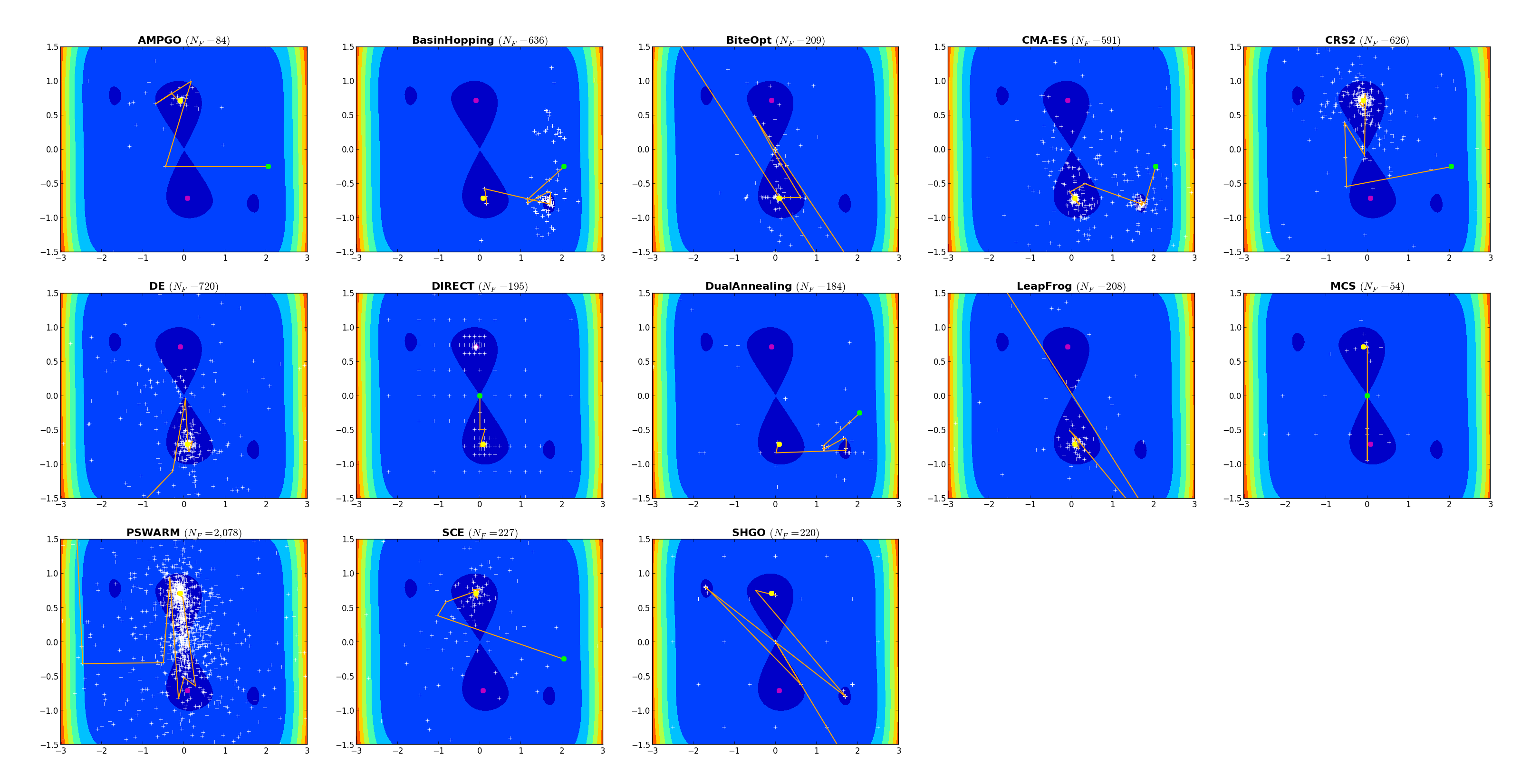
Figure 0.7: Solver search progress for test problem Six Humps Camel Back function

The Benchmarks¶

Stopping Conditions and Tolerances¶

High-Level Description of the Test Suites¶