Schoen¶

F_opt Known	X_opt Known	Difficulty
Yes	Yes	Easy

The Schoen generator is a benchmark generator for essentially unconstrained global optimization test functions. It is based on the early work of Fabio Schoen and his short note on a simple but interesting idea on a test function generator.

Many thanks go to Professor Fabio Schoen for providing an updated copy of the source code and for the email communications.

Methodology¶

The main advantages of functions belonging to the Schoen generator are:

They are easily built for any dimension
Their global minimum and maximum are known a priori
Their smoothness is controllable by means of a set of parameters
The number and location of stationary points is controllable by the user

The definition of the test functions is the following:

$f(x) = \frac{\sum_{i=1}^{k} f_i \prod_{j \neq i} \left \| x - z_j \right \|^{\alpha_j} }{\sum_{i=1}^{k} \prod_{j \neq i} \left \| x - z_j \right \|^{\alpha_j}}$

Where:

$x \in [0, 1)^N$
$k \in \mathbb{N}$
$z_j \in [0, 1]^N, \: \: \forall j=1, ..., k$
$f_i \in \mathbb{R}, \: \: \forall i=1, ..., k$
$\alpha_i \in \mathbb{R}^+, \: \: \forall i=1, ..., k$

and the norm used is the euclidean norm (although different norms might be used as well). The main properties of these functions are the following:

$\: \: f(z_i) = f_i , \: \: \forall i=1, ..., k$
$\: \: \min_{i=1,k} f_i \leq f(x) \leq \max_{i=1,k} f_i , \: \: \forall i=1, ..., k$
$\: \: \textup{If} \: \: \alpha_i > 1, \textup{then} \: \: \lim_{x \mapsto z_i } \nabla f(x) = 0$
$\: \: \textup{If} \: \: \alpha_i > 1, \textup{then} \: \: f(x) - f(z_i) = \emph{O}(\left \| x - z_j \right \|^{\alpha_i})$

I have taken the C code in the note and converted it into Python, thus creating 285 benchmark functions with dimensionality ranging from 2 to 6.

A few examples of 2D benchmark functions created with the Schoen generator can be seen in Figure 15.1.

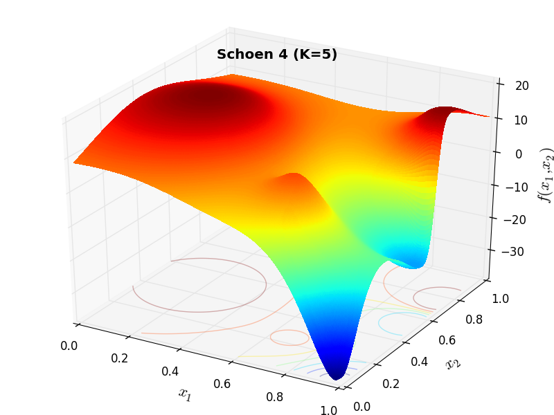
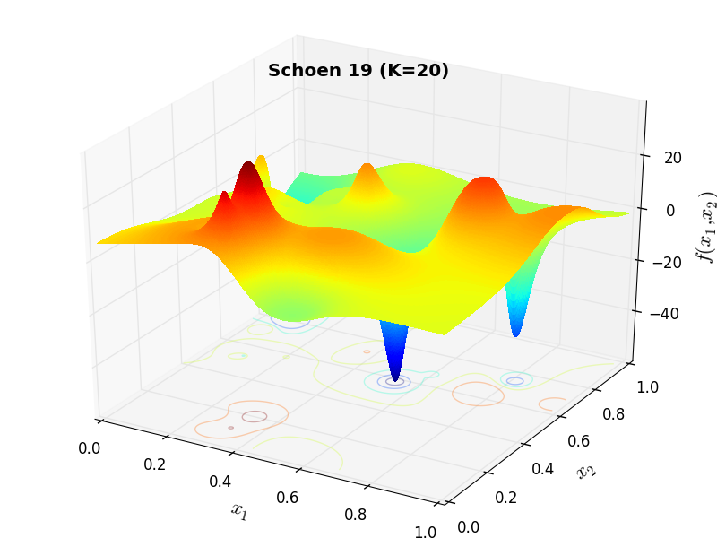
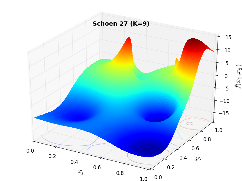
Schoen Function 4	Schoen Function 19	Schoen Function 27
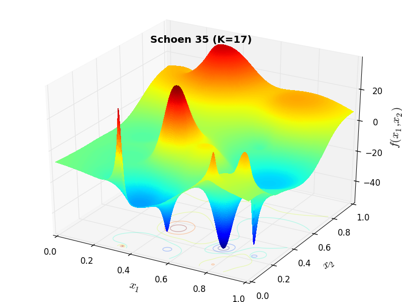
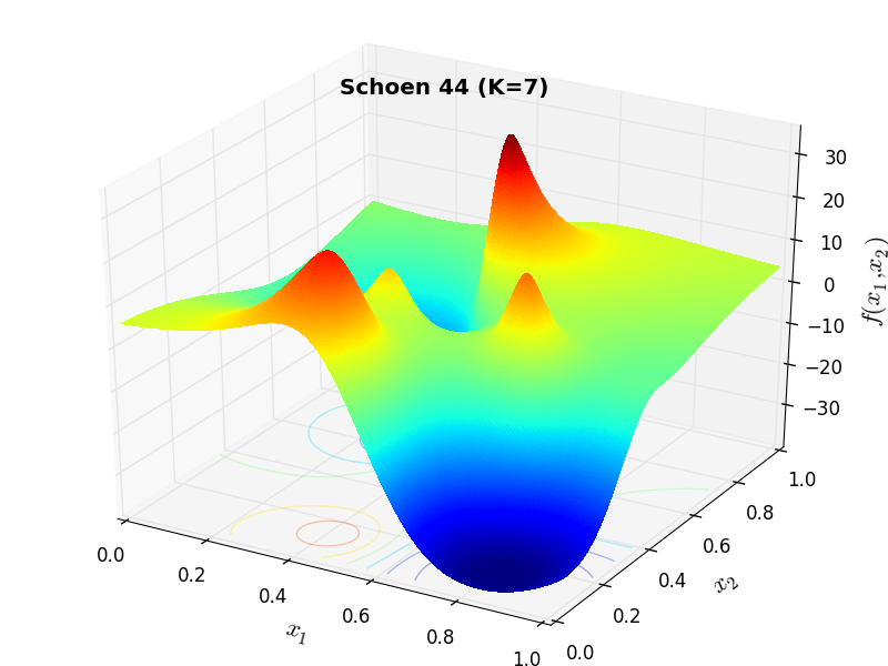
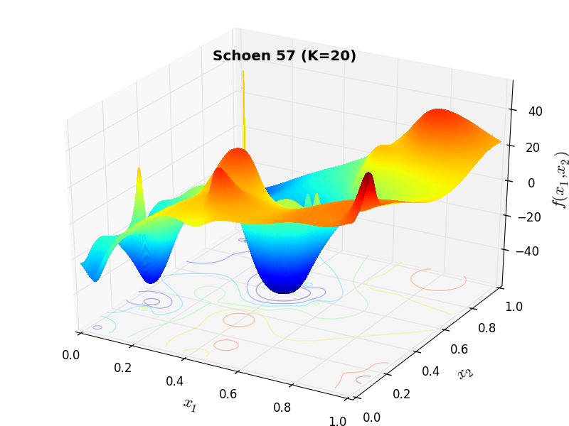
Schoen Function 35	Schoen Function 44	Schoen Function 57

General Solvers Performances¶

Table 15.1 below shows the overall success of all Global Optimization algorithms, considering every benchmark function, for a maximum allowable budget of $NF = 2,000$ .

The Schoen benchmark suite is a very easy test suite: the best solver for $NF = 2,000$ is SHGO, with a success rate of 95.4%, but many solvers are able to find more than 75% of global minima: MCS, DIRECT, BasinHopping, and DualAnnealing.

Note

The reported number of functions evaluations refers to successful optimizations only.

**Table 15.1**: Solvers performances on the Schoen benchmark suite at NF = 2,000
Optimization Method	Overall Success (%)	Functions Evaluations
AMPGO	53.33%	278
BasinHopping	90.18%	307
BiteOpt	70.53%	286
CMA-ES	71.23%	540
CRS2	67.37%	822
DE	52.28%	1,393
DIRECT	75.44%	313
DualAnnealing	85.61%	159
LeapFrog	52.63%	303
MCS	91.23%	276
PSWARM	58.25%	1,291
SCE	68.42%	391
SHGO	95.44%	267

These results are also depicted in Figure 15.2, which shows that SHGO is the better-performing optimization algorithm, followed by very many other solvers with similar performances.

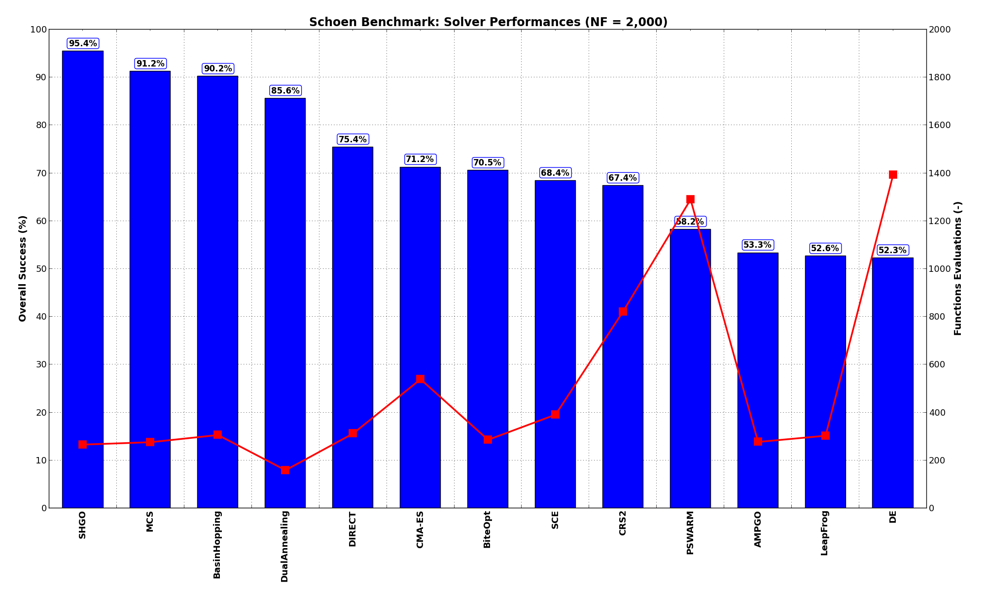
Optimization algorithms performances on the Schoen test suite at :math:`NF = 2,000`

Figure 15.2: Optimization algorithms performances on the Schoen test suite at $NF = 2,000$

Pushing the available budget to a very generous $NF = 10,000$ , the results show MCS snatching the top spot from SHGO, although the two algorithms are so close to be virtually equuivalent in performances. BasinHopping and AMPGO do also quite well with more than 90% rate of success. The results are also shown visually in Figure 15.3.

**Table 15.2**: Solvers performances on the Schoen benchmark suite at NF = 10,000
Optimization Method	Overall Success (%)	Functions Evaluations
AMPGO	90.53%	2,178
BasinHopping	95.09%	498
BiteOpt	74.39%	576
CMA-ES	78.95%	871
CRS2	69.82%	904
DE	74.39%	2,337
DIRECT	83.51%	756
DualAnnealing	87.72%	228
LeapFrog	52.63%	303
MCS	96.84%	485
PSWARM	71.93%	1,571
SCE	69.47%	437
SHGO	96.14%	297

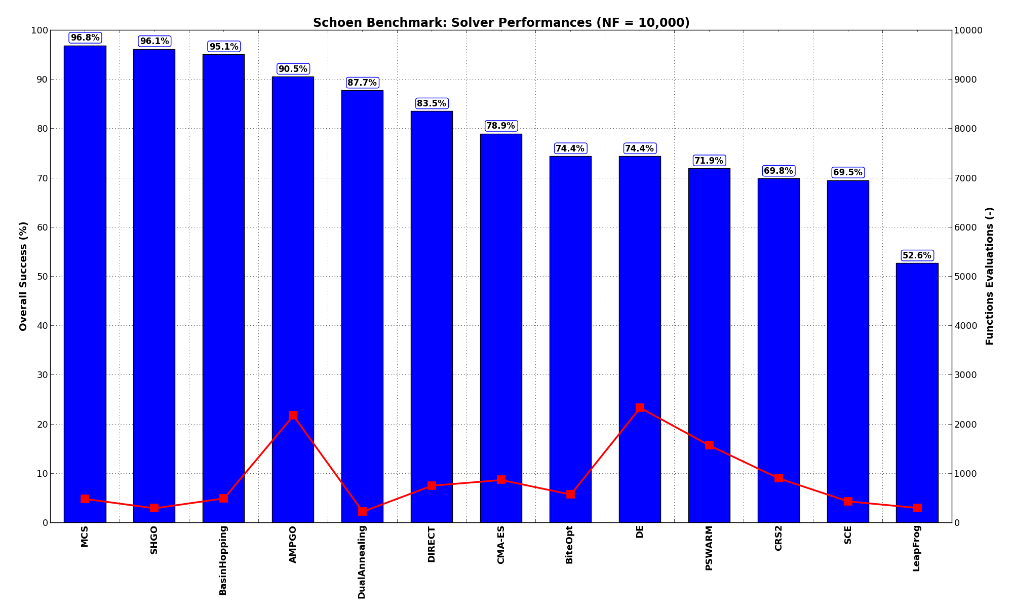
Optimization algorithms performances on the Schoen test suite at :math:`NF = 10,000`

Figure 15.3: Optimization algorithms performances on the Schoen test suite at $NF = 10,000$

Sensitivities on Functions Evaluations Budget¶

It is also interesting to analyze the success of an optimization algorithm based on the fraction (or percentage) of problems solved given a fixed number of allowed function evaluations, let’s say 100, 200, 300,... 2000, 5000, 10000.

In order to do that, we can present the results using two different types of visualizations. The first one is some sort of “small multiples” in which each solver gets an individual subplot showing the improvement in the number of solved problems as a function of the available number of function evaluations - on top of a background set of grey, semi-transparent lines showing all the other solvers performances.

This visual gives an indication of how good/bad is a solver compared to all the others as function of the budget available. Results are shown in Figure 15.4.

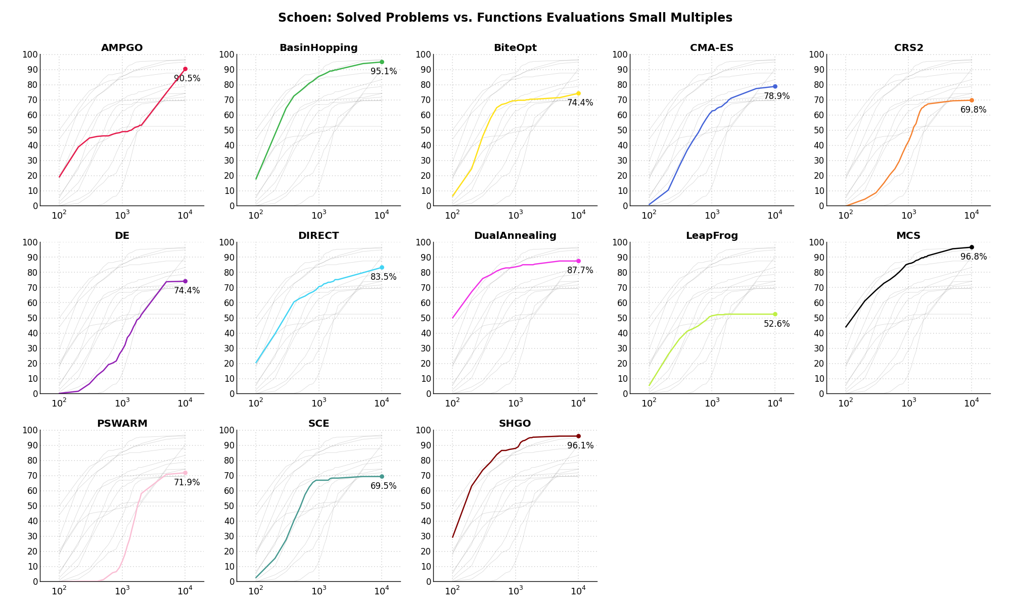
Figure 15.4: Percentage of problems solved given a fixed number of function evaluations on the Schoen test suite

The second type of visualization is sometimes referred as “Slopegraph” and there are many variants on the plot layout and appearance that we can implement. The version shown in Figure 15.5 aggregates all the solvers together, so it is easier to spot when a solver overtakes another or the overall performance of an algorithm while the available budget of function evaluations changes.

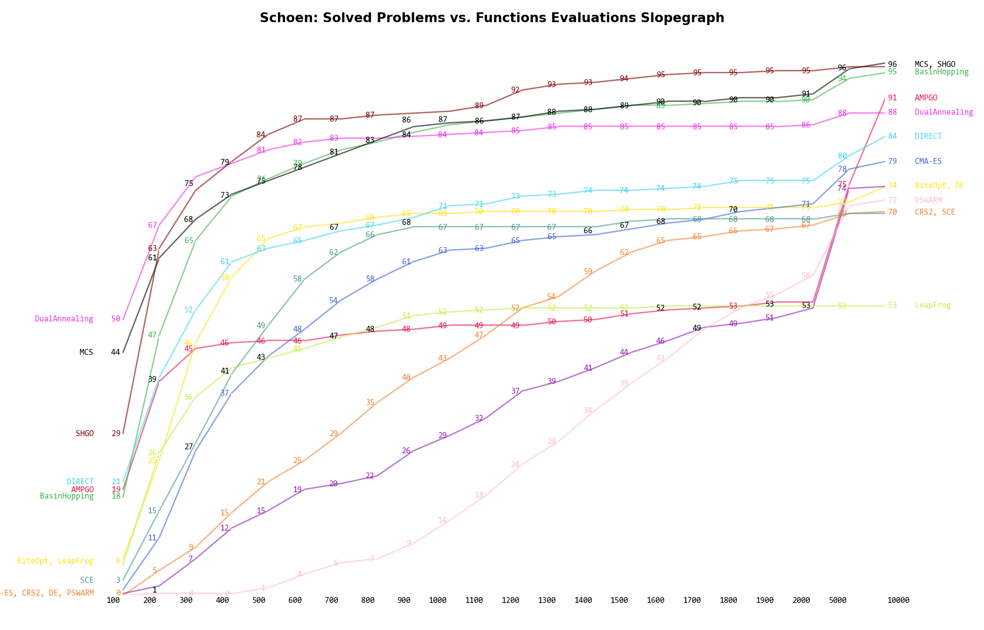
Figure 15.5: Percentage of problems solved given a fixed number of function evaluations on the Schoen test suite

A few obvious conclusions we can draw from these pictures are:

For this specific benchmark test suite, for very small budgets (i.e., $NF < 500$ ) DualAnnealing appears to be the most successful solver.
For more generous number of fucntions evaluations, SHGO is pretty much unbeatable un until very large budgets, where MCS takes the lead. BasinHopping has also a very high rate of success.
AMPGO displays an enormous ramp up in solved problems for very large number of function evaluations.

Dimensionality Effects¶

Since I used the Schoen test suite to generate test functions with dimensionality ranging from 2 to 6, it is interesting to take a look at the solvers performances as a function of the problem dimensionality. Of course, in general it is to be expected that for larger dimensions less problems are going to be solved - although it is not always necessarily so as it also depends on the function being generated. Results are shown in Table 15.3 .

**Table 15.3**: Dimensionality effects on the Schoen benchmark suite at NF = 2,000
Solver	N = 2	N = 3	N = 4	N = 5	N = 6	Overall
AMPGO	61.4	52.6	57.9	47.4	47.4	53.3
BasinHopping	94.7	93.0	84.2	87.7	91.2	90.2
BiteOpt	78.9	68.4	66.7	71.9	66.7	70.5
CMA-ES	71.9	73.7	70.2	75.4	64.9	71.2
CRS2	63.2	66.7	71.9	73.7	61.4	67.4
DE	77.2	73.7	68.4	42.1	0.0	52.3
DIRECT	94.7	84.2	77.2	63.2	57.9	75.4
DualAnnealing	91.2	82.5	82.5	89.5	82.5	85.6
LeapFrog	59.6	54.4	57.9	54.4	36.8	52.6
MCS	96.5	96.5	89.5	93.0	80.7	91.2
PSWARM	86.0	66.7	61.4	47.4	29.8	58.2
SCE	75.4	70.2	68.4	68.4	59.6	68.4
SHGO	100.0	100.0	94.7	94.7	87.7	95.4

Figure 15.6 shows the same results in a visual way.

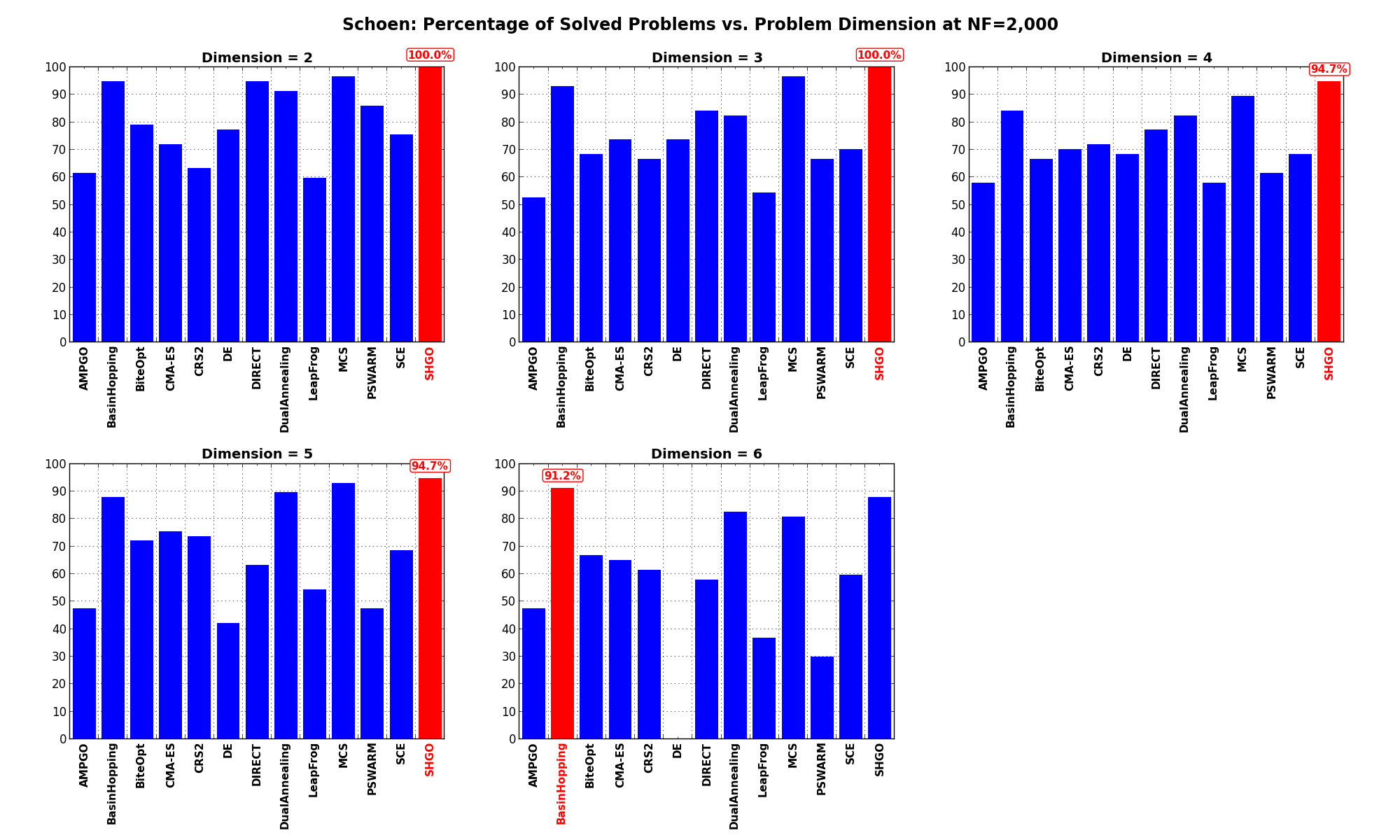
Percentage of problems solved as a function of problem dimension at :math:`NF = 2,000`

Figure 15.6: Percentage of problems solved as a function of problem dimension for the Schoen test suite at $NF = 2,000$

What we can infer from the table and the figure is that, for low dimensionality problems ( $N \leq 3$ ), SHGO has the perfect score of 100%, solving all problems, tightly followed by MCS, DualAnnealing and BasinHopping. By increasing the dimensionality the trend doesn’t change much, although BasinHopping manages to take the load for higher dimensions ( $N = 6$ ).

Pushing the available budget to a very generous $NF = 10,000$ shows MCS taking the lead in general, although SHGO and BasinHopping still behave astonishingly well.

The results for the benchmarks at $NF = 10,000$ are displayed in Table 15.4 and Figure 15.7.

**Table 15.4**: Dimensionality effects on the Schoen benchmark suite at NF = 10,000
Solver	N = 2	N = 3	N = 4	N = 5	N = 6	Overall
AMPGO	93.0	96.5	91.2	91.2	80.7	90.5
BasinHopping	96.5	96.5	87.7	96.5	98.2	95.1
BiteOpt	84.2	75.4	71.9	73.7	66.7	74.4
CMA-ES	75.4	75.4	78.9	84.2	80.7	78.9
CRS2	66.7	66.7	71.9	73.7	70.2	69.8
DE	77.2	73.7	71.9	78.9	70.2	74.4
DIRECT	96.5	91.2	80.7	80.7	68.4	83.5
DualAnnealing	93.0	89.5	82.5	89.5	84.2	87.7
LeapFrog	59.6	54.4	57.9	54.4	36.8	52.6
MCS	98.2	100.0	96.5	96.5	93.0	96.8
PSWARM	87.7	71.9	71.9	68.4	59.6	71.9
SCE	77.2	70.2	70.2	68.4	61.4	69.5
SHGO	100.0	100.0	94.7	98.2	87.7	96.1

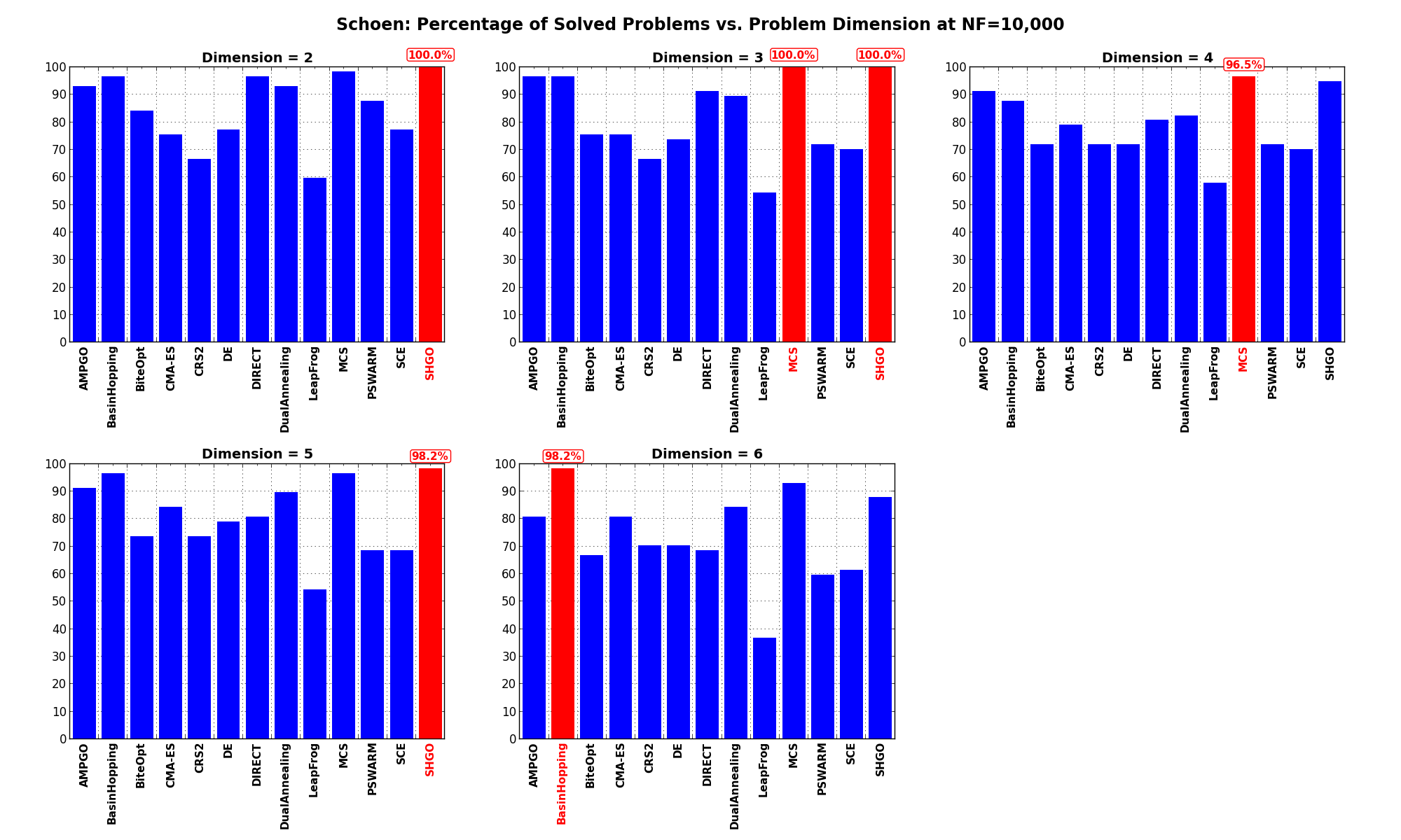
Percentage of problems solved as a function of problem dimension at :math:`NF = 10,000`

Figure 15.7: Percentage of problems solved as a function of problem dimension for the Schoen test suite at $NF = 10,000$

Schoen¶

Methodology¶

General Solvers Performances¶

Sensitivities on Functions Evaluations Budget¶

Dimensionality Effects¶

Table Of Contents

Previous topic

Next topic

This Page

Navigation

Schoen¶

Methodology¶

General Solvers Performances¶

Sensitivities on Functions Evaluations Budget¶

Dimensionality Effects¶

Table Of Contents

Previous topic

Next topic

This Page

Quick search

Navigation