Navigation
- index
- next |
- previous |

- Home »
- The Benchmarks »
- NLSE
 NLSE
NLSE¶| Fopt Known | Xopt Known | Difficulty |
|---|---|---|
| Yes | Yes | Easy |
The realm of nonlinear systems of equations is not 100% tailored to global optimization algorithms; nevertheless, nothing stops you from applying a global solver to try and optimize a system of nonlinear equations, assuming the formulation is appropriate for the solvers.
 Methodology
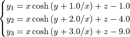
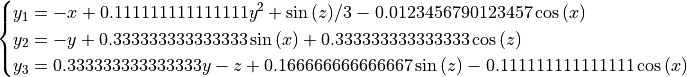
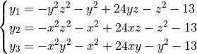
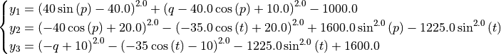
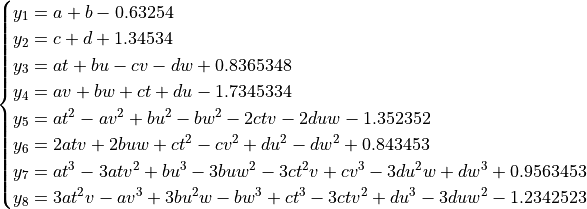
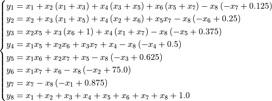
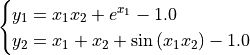
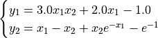
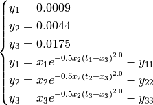
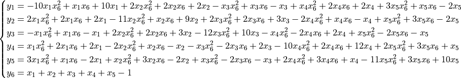
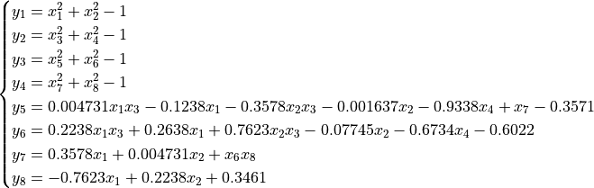
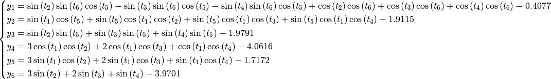
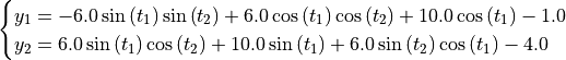
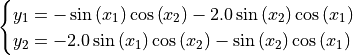
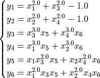
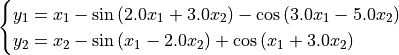
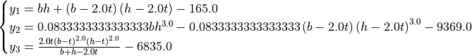
In order to build this dataset I have drawn from many different sources (Publications, ALIAS/COPRIN and many others) to create 44 systems of nonlinear equations with dimensionality ranging from 2 to 8. A complete set of formulas giving the actual equations is presented in the section NLSE Datasets, and specifically in Table 14.4 .
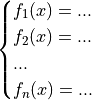
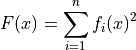
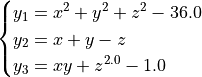
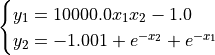
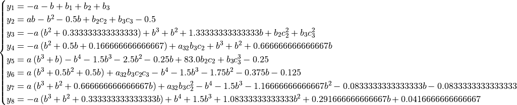
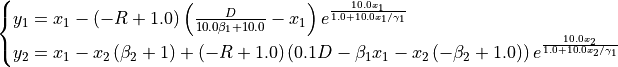
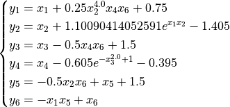
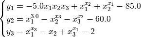
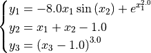
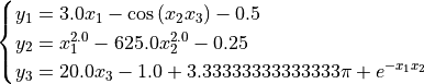
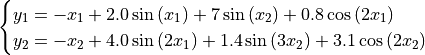
The approach for building a single-valued objective function out of a system of nonlinear equations:
Is to treat it kind of like a nonlinear least squares problem, where the actual (scalar-valued) objective function is easily formulated as:
Then, of course, the global minimum is attained at  .
.
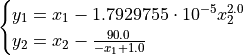
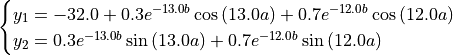
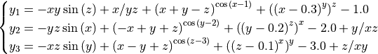
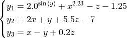
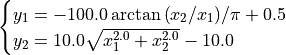
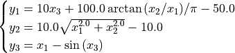
A few examples of 2D benchmark functions created with the NLSE test suite can be seen in Figure 14.1.
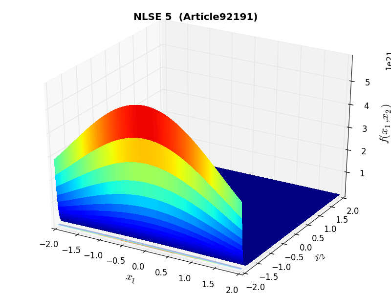
NLSE Function Article92191 |
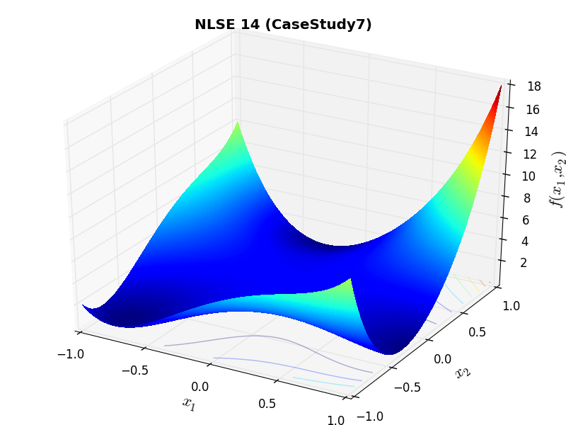
NLSE Function CaseStudy7 |
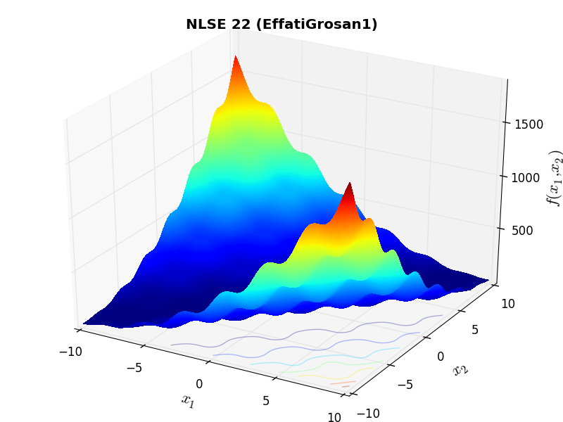
NLSE Function EffatiGrosan1 |
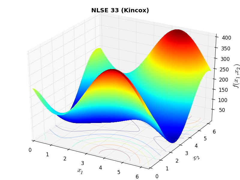
NLSE Function Kincox |
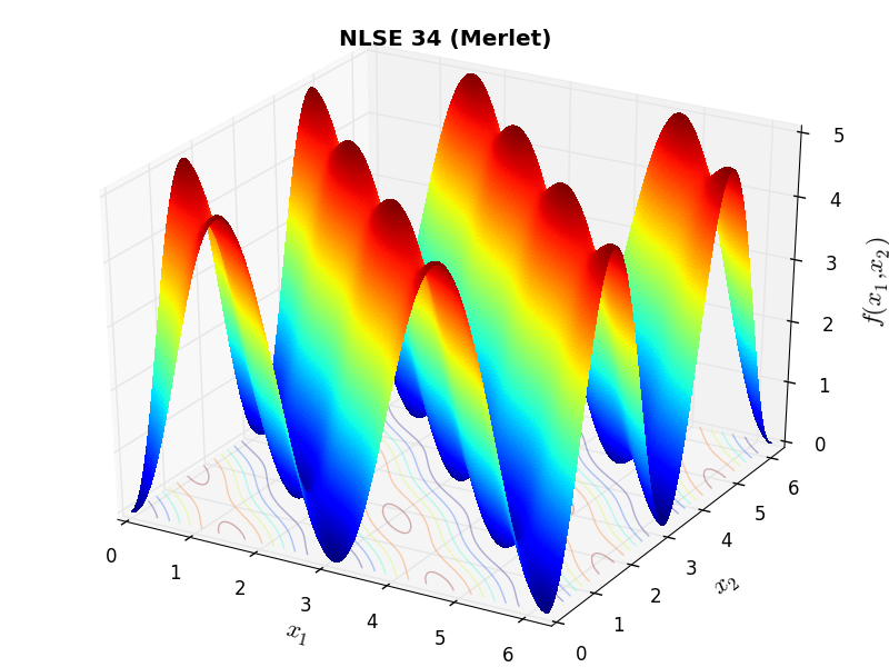
NLSE Function Merlet |
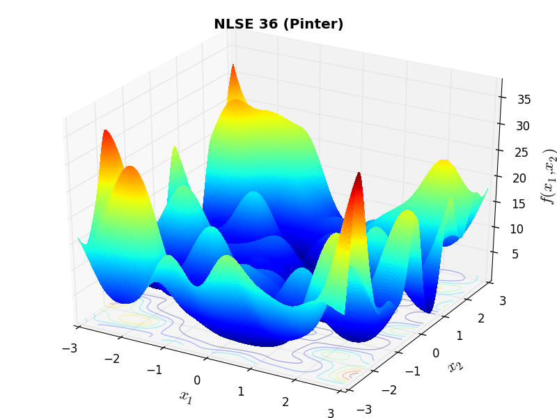
NLSE Function Pinter |
 General Solvers Performances
Table 14.1 below shows the overall success of all Global Optimization algorithms, considering every benchmark function,
for a maximum allowable budget of  .
.
The NLSE benchmark suite is an easy test suite: the best solver for is MCS, with a success
rate of 79.6%, but many solvers are able to correctly optimize more than 60% of objectiv functions:: BiteOpt, AMPGO, SHGO,
BasinHopping and SCE.
Note
The reported number of functions evaluations refers to successful optimizations only.
| Optimization Method | Overall Success (%) | Functions Evaluations |
|---|---|---|
| AMPGO | 63.64% | 321 |
| BasinHopping | 63.64% | 342 |
| BiteOpt | 75.00% | 490 |
| CMA-ES | 52.27% | 622 |
| CRS2 | 38.64% | 801 |
| DE | 45.45% | 1,234 |
| DIRECT | 47.73% | 433 |
| DualAnnealing | 56.82% | 132 |
| LeapFrog | 54.55% | 412 |
| MCS | 79.55% | 195 |
| PSWARM | 27.27% | 1,215 |
| SCE | 61.36% | 811 |
| SHGO | 65.91% | 257 |
These results are also depicted in Figure 14.2, which shows that MCS is the better-performing optimization algorithm, followed by very many other solvers with similar performances.
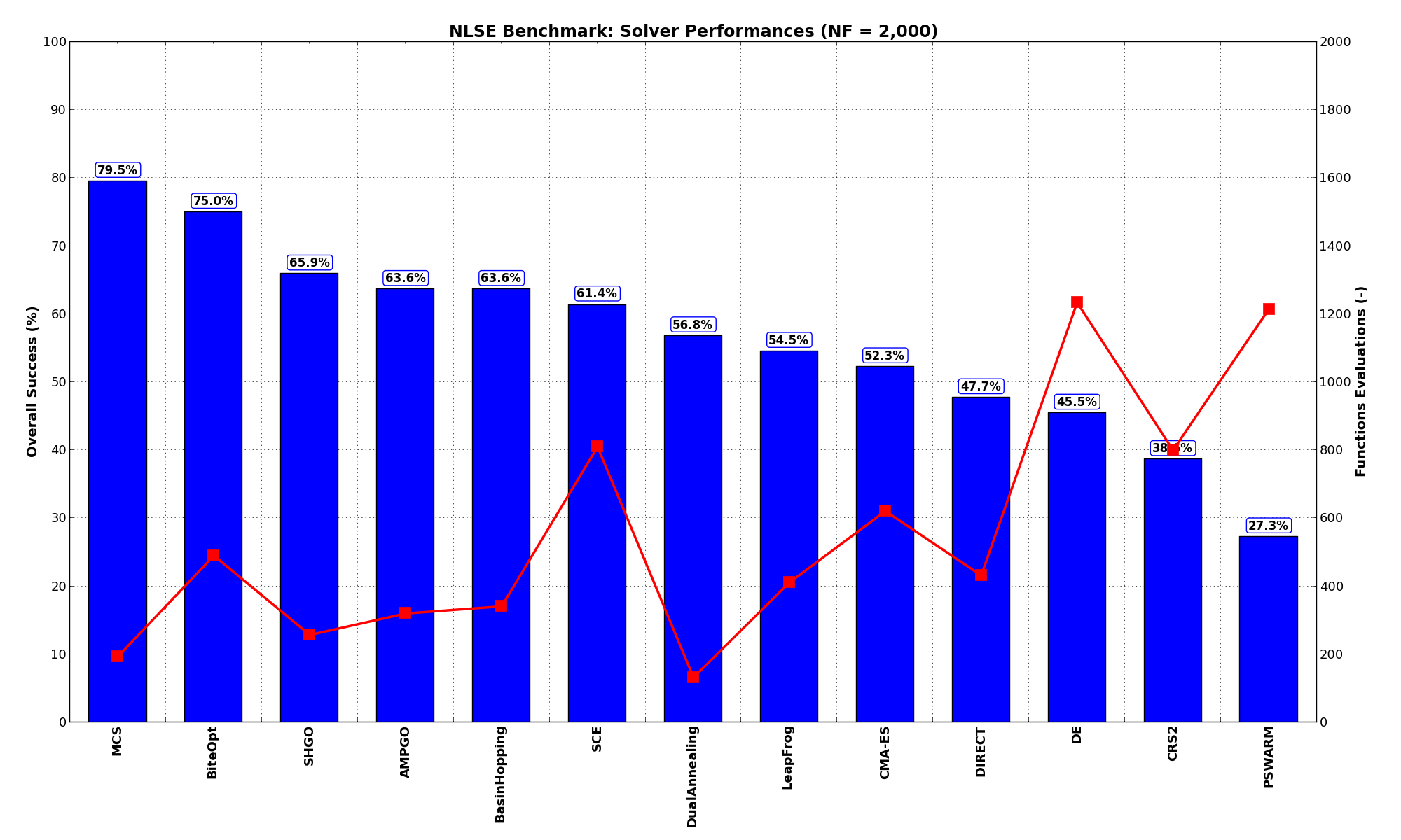
Figure 14.2: Optimization algorithms performances on the NLSE test suite at
Pushing the available budget to a very generous 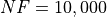 , the results show MCS basically solving all
the problems at a 95.5% success rate, with BiteOpt now much closer and AMPGO trailing in third place.
The results are also shown visually in Figure 14.3.
, the results show MCS basically solving all
the problems at a 95.5% success rate, with BiteOpt now much closer and AMPGO trailing in third place.
The results are also shown visually in Figure 14.3.
| Optimization Method | Overall Success (%) | Functions Evaluations |
|---|---|---|
| AMPGO | 75.00% | 999 |
| BasinHopping | 68.18% | 683 |
| BiteOpt | 90.91% | 1,061 |
| CMA-ES | 59.09% | 1,146 |
| CRS2 | 52.27% | 1,645 |
| DE | 65.91% | 2,306 |
| DIRECT | 52.27% | 974 |
| DualAnnealing | 61.36% | 373 |
| LeapFrog | 65.91% | 1,234 |
| MCS | 95.45% | 910 |
| PSWARM | 54.55% | 2,423 |
| SCE | 68.18% | 970 |
| SHGO | 65.91% | 257 |
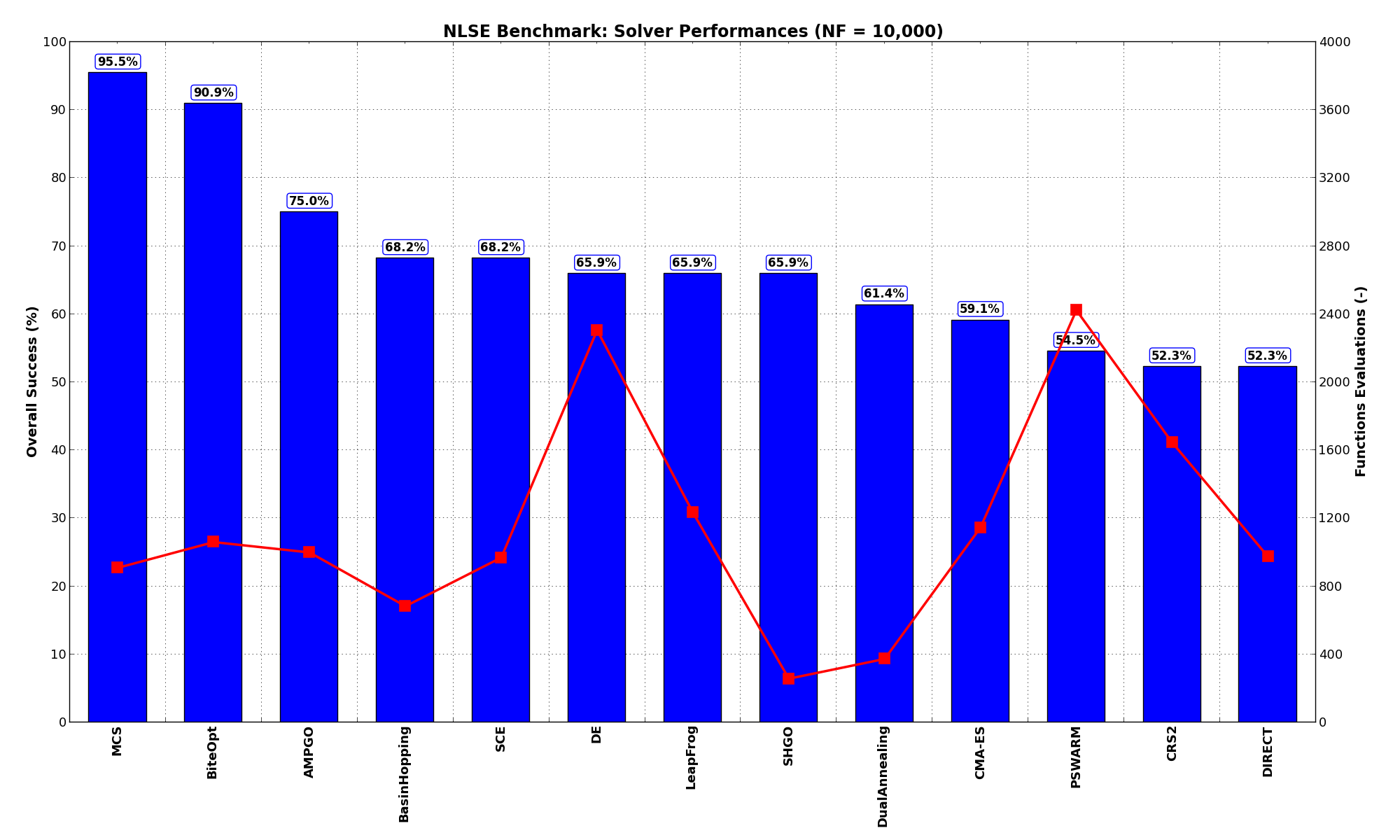
Figure 14.3: Optimization algorithms performances on the NLSE test suite at
 Sensitivities on Functions Evaluations Budget
It is also interesting to analyze the success of an optimization algorithm based on the fraction (or percentage) of problems solved given a fixed number of allowed function evaluations, let’s say 100, 200, 300,... 2000, 5000, 10000.
In order to do that, we can present the results using two different types of visualizations. The first one is some sort of “small multiples” in which each solver gets an individual subplot showing the improvement in the number of solved problems as a function of the available number of function evaluations - on top of a background set of grey, semi-transparent lines showing all the other solvers performances.
This visual gives an indication of how good/bad is a solver compared to all the others as function of the budget available. Results are shown in Figure 14.4.
Figure 14.4: Percentage of problems solved given a fixed number of function evaluations on the NLSE test suite
The second type of visualization is sometimes referred as “Slopegraph” and there are many variants on the plot layout and appearance that we can implement. The version shown in Figure 14.5 aggregates all the solvers together, so it is easier to spot when a solver overtakes another or the overall performance of an algorithm while the available budget of function evaluations changes.
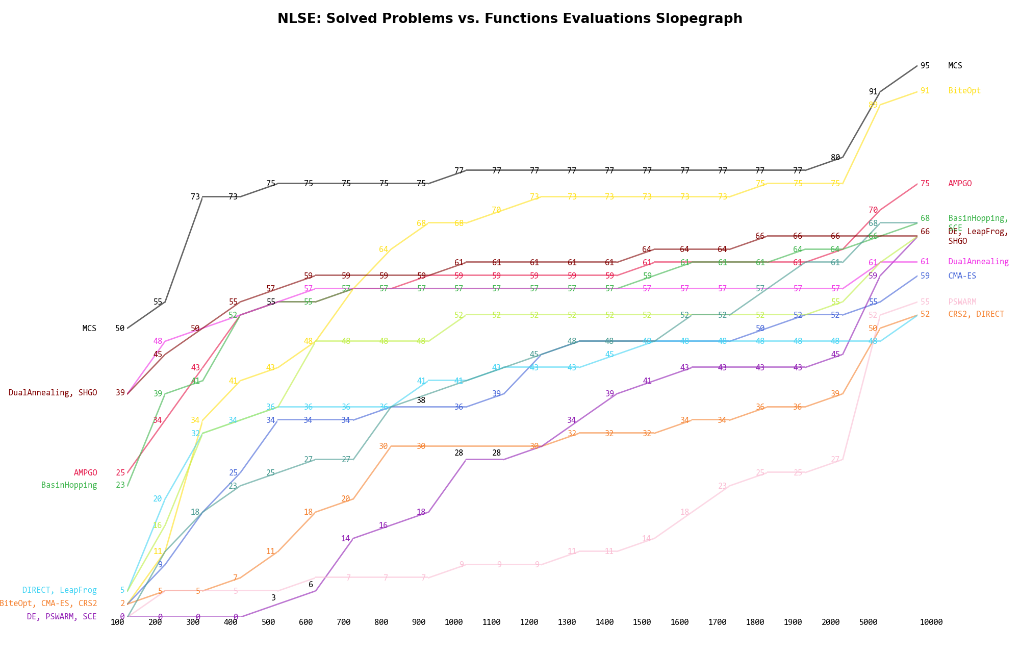
Figure 14.5: Percentage of problems solved given a fixed number of function evaluations on the NLSE test suite
A few obvious conclusions we can draw from these pictures are:
 NLSE Datasets
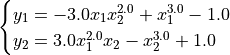
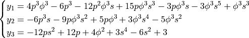
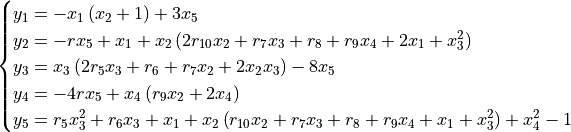
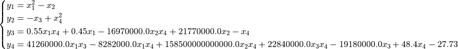
| Name | Dimension | Function |
|---|---|---|
| AOLcosh1 | 3 |
|
| Article89741 | 3 |
|
| Article90897 | 2 |
|
| Article92191 | 2 |
|
| Auto2Fit1 | 3 |
|
| Auto2Fit2 | 3 |
|
| Bronstein | 3 |
|
| Bullard | 2 |
|
| Butcher8 | 8 |
|
| CSTR | 2 |
|
| CaseStudy3 | 6 |
|
| CaseStudy4 | 3 |
|
| CaseStudy5 | 3 |
|
| CaseStudy6 | 3 |
|
| CaseStudy7 | 2 |
|
| Celestial | 3 |
|
| Chem | 5 |
|
| Chemk | 4 |
|
| Cyclo | 3 |
|
| DiGregorio | 3 |
|
| Dipole | 8 |
|
| Eco9 | 8 |
|
| EffatiGrosan1 | 2 |
|
| EffatiGrosan2 | 2 |
|
| F3 | 2 |
|
| Ferrais | 2 |
|
| Gaussian | 3 |
|
| GenEig | 6 |
|
| Helical | 2 |
|
| Helical1 | 3 |
|
| Kearl11 | 8 |
|
| Kin1 | 6 |
|
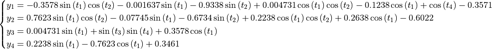
| Kincox | 2 |
|
| Merlet | 2 |
|
| Neuro | 6 |
|
| Pinter | 2 |
|
| Puma | 4 |
|
| Semiconductor | 6 |
|
| SixBody | 6 |
|
| SjirkBoon | 4 |
|
| ThinWall | 3 |
|
| Xu | 2 |
|