MCS

Multilevel Coordinate Search (MCS) is an efficient algorithm for bound constrained global optimization using function values only.

To do so, the -dimensional search space is represented by a set of non-intersecting hypercubes (boxes). The boxes are then iteratively split along an axis plane according to the value of the function at a representative point of the box (and its neighbours) and the box’s size. These two splitting criteria combine to form a global search by splitting large boxes and a local search by splitting areas for which the function value is good.

Additionally, a local search combining a (multi-dimensional) quadratic interpolant of the function and line searches can be used to augment performance of the algorithm (MCS with local search); in this case the plain MCS is used to provide the starting (initial) points. The information provided by local searches (namely local minima of the objective function) is then fed back to the optimizer and influences the splitting criteria, resulting in reduced sample clustering around local minima and faster convergence.

Simplified workflow

The basic workflow is presented in Figure 17.1. Generally, each step can be characterized by three stages:

1. Identify a potential candidate for splitting (magenta, thick).
2. Identify the optimal splitting direction and the expected optimal position of splitting points (green).
3. Evaluate the objective function at splitting points not considered previously. Generate new boxes (magenta, thin) based on the values of the objective function at splitting (green) points.

At every step at least one splitting point (yellow) is a known function sample (red) hence the objective is never evaluated there again.

In order to determine if a box will be split two separate splitting criteria are used. The first one, splitting by rank, ensures that large boxes that have not been split too often will be split eventually. If it applies then the splitting point can be determined a priori. The second one, splitting by expected gain, employs a local one-dimensional quadratic model (surrogate) along a single coordinate. In this case the splitting point is defined as the minimum of the surrogate and the box is split only if the interpolant value there is lower than the current best sampled function value.

Figure 17.1: MCS algorithm (without local search) applied to the two-dimensional Rosenbrock function

Convergence

The algorithm is guaranteed to converge to the global minimum in the long run (i.e. when the number of function evaluations and the search depth are arbitrarily large) if the objective function is continuous in the neighbourhood of the global minimizer. This follows from the fact that any box will become arbitrarily small eventually, hence the spacing between samples tends to zero as the number of function evaluations tends to infinity.

Recursive implementation

MCS was designed to be implemented in an efficient recursive way with the aid of trees. With this approach the amount of memory required is independent of problem dimensionality since the sampling points are not stored explicitly. Instead, just a single coordinate of each sample is saved and the remaining coordinates can be recovered by tracing the history of a box back to the root (initial box). This method was suggested by the authors and used in their original implementation.

When implemented carefully this also allows for avoiding repeated function evaluations. More precisely, if a sampling point is placed along the boundary of two adjacent boxes then this information can often be extracted through backtracing the point’s history for a small number of steps. Consequently, new subboxes can be generated without evaluating the (potentially expensive) objective function. This scenario is visualised in figure 1 whenever a green (but not yellow) and a red point coincide e.g. when the box with corners around and is split.

Methodology

The Python implementation is my translation to Python of the original Matlab code from A. Neumaier and W. Huyer (giving then for free also GLS and MINQ):

https://www.mat.univie.ac.at/~neum/software/mcs/

I have added a few, minor improvements compared to the original implementation.

In order to test the correctess of my implementation, I have run the Matlab and Python code on dozens of objective functions, thus testing also the implementations of GLS and MINQ5. What follows is a subset of results obtained and it is presented as a validation of the implementation itself.

For some selected, very famous multi-modal test functions, I have forced the Matlab and Python codes to stop when the absolute difference between the global optimum and the best function value was less than . Figure 17.2 shows some data in terms of convergence results and number of function evaluations.

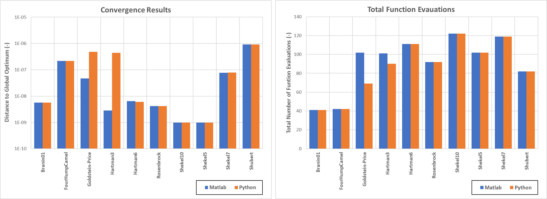
Figure 17.2: Convergence results and function evaluations for the Matlab/Python MCS implementations

As can be seen, the Matlab and Python implementations give the same results, up to extremely small numbers in terms of convergence criteria. This is due to the behaviour of the local search in the GLS/MINQ5 routines, as highlighted in Figure 17.3 .

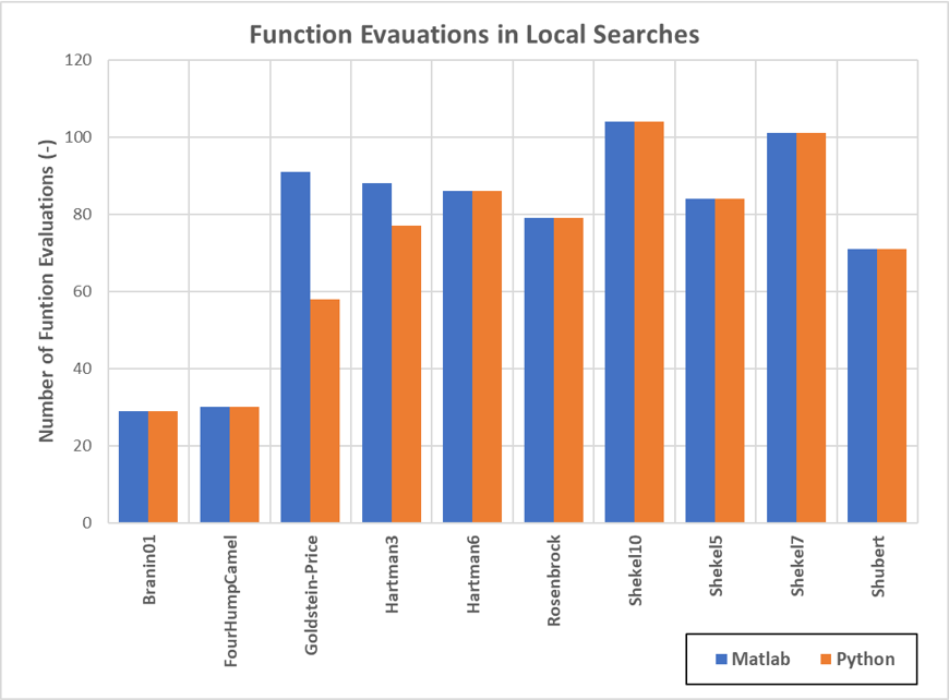
Figure 17.3: Local optimization through GLS/MINQ5 in Matlab/Python

After painstaking debugging, I have tracked down that the differences are due to slightly different outputs in the matrix linear algebra, and specifically marginally different results obtained through the Matlab backslash operator and the NumPy linalg solve algorithm.