CVMG¶

F_opt Known	X_opt Known	Difficulty
Yes	No	Medium

This benchmark test suite represents yet another “landscape generator”, I had to dig it out using the Wayback Machine at http://web.archive.org/web/20100612044104/https://www.cs.uwyo.edu/~wspears/multi.kennedy.html . The acronym stands for “Continuous Valued Multimodality Generator”. The source code is in C++ but it’s fairly easy to port it to Python.

In addition to the original implementation (that uses the Sigmoid as a softmax/transformation function) I have added a few others to create varied landscapes.

Methodology¶

The objective functions in this test suite are relatively easy to generate. By selecting a number of desired peaks ( $N_p$ ) and the problem dimension ( $d$ ) we can define a “landscape” function as:

$L = k \cdot \mathcal{U}(N_p, d)$

Where $k$ is a user-selectable constant and $\mathcal{U}$ is the uniform distribution over $[0, 1)$ .

Then, through the use of a softmax/transformation function $S$ (which can be a sigmoid, or tanh or arctan, etc..., whatever input vector of parameters ( $x$ ) is restricted in the interval $[-1, 1]$ , with a function $T$ like:

$T(x) = k \cdot S(x)$

Finally, the objective function is defined as:

$F(x) = \textbf{min} \left [ \sum_{i=1}^d (S(x) - L)^2 \right ] + 1$

That said, my approach to generate test functions for this benchmark has been the following:

The dimensionality of the problem varies between $N = 2$ and $N = 5$
The number of peaks can be any of 10, 30, 50, 70, 90.
The multiplier $k$ can be 1, 5, or 10
The softmax/transformation function can be one of “sigmoid”, “algebraic”, “tanh”, “arctan”, “absolute”, “gd” - their shape is explained in Wikipedia .

With all these variable settings, I generated 90 valid test function per dimension, thus the current CVMG test suite contains 360 benchmark functions, with dimensionality ranging from 2 to 5.

A few examples of 2D benchmark functions created with the CVMG generator can be seen in Figure 13.1.

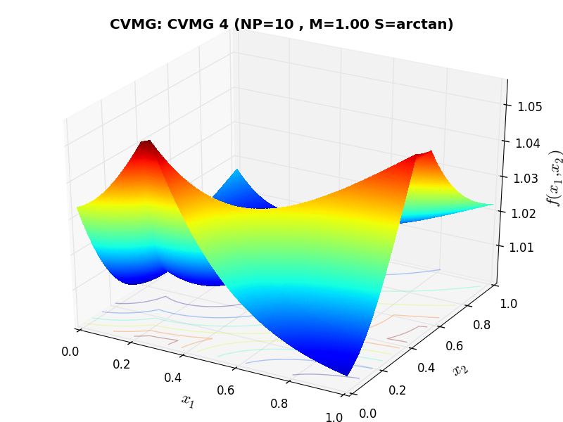
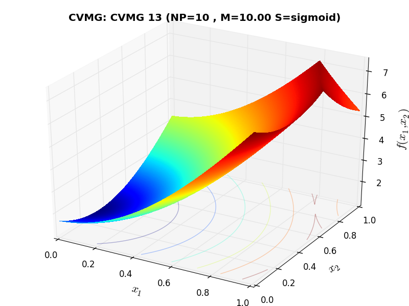
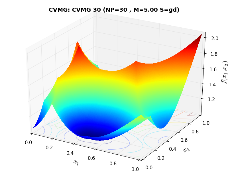
CVMG Function 4	CVMG Function 13	CVMG Function 30
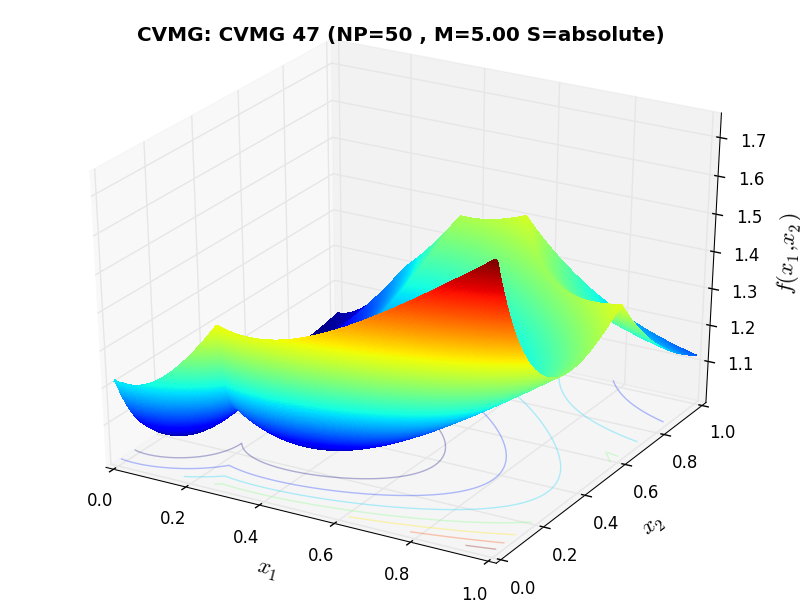
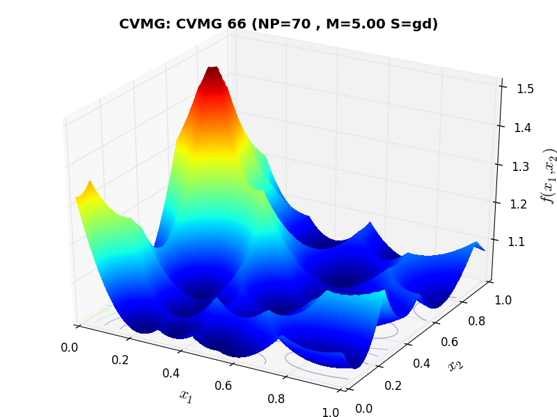
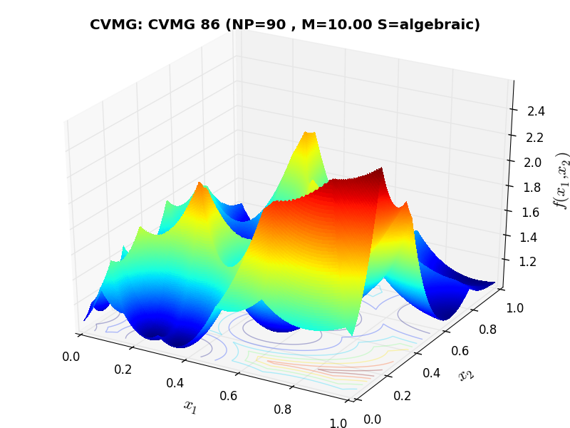
CVMG Function 47	CVMG Function 66	CVMG Function 86

General Solvers Performances¶

Table 13.1 below shows the overall success of all Global Optimization algorithms, considering every benchmark function, for a maximum allowable budget of $NF = 2,000$ .

The CVMG benchmark suite is a medium-difficulty test suite: the best solver for $NF = 2,000$ is MCS, with a success rate of 56.4%, but many solvers are close to that performance: DIRECT, BasinHopping, SHGO, DualAnnealing and AMPGO all stand between 3% to the top optimization algorithm.

Note

The reported number of functions evaluations refers to successful optimizations only.

**Table 13.1**: Solvers performances on the CVMG benchmark suite at NF = 2,000
Optimization Method	Overall Success (%)	Functions Evaluations
AMPGO	53.89%	252
BasinHopping	55.00%	155
BiteOpt	47.22%	263
CMA-ES	50.83%	424
CRS2	40.56%	683
DE	48.33%	1,069
DIRECT	55.56%	185
DualAnnealing	54.17%	119
LeapFrog	42.50%	184
MCS	56.39%	106
PSWARM	41.94%	1,369
SCE	50.56%	435
SHGO	54.72%	130

These results are also depicted in Figure 13.2, which shows that MCS is the better-performing optimization algorithm, followed by very many other solvers with similar performances.

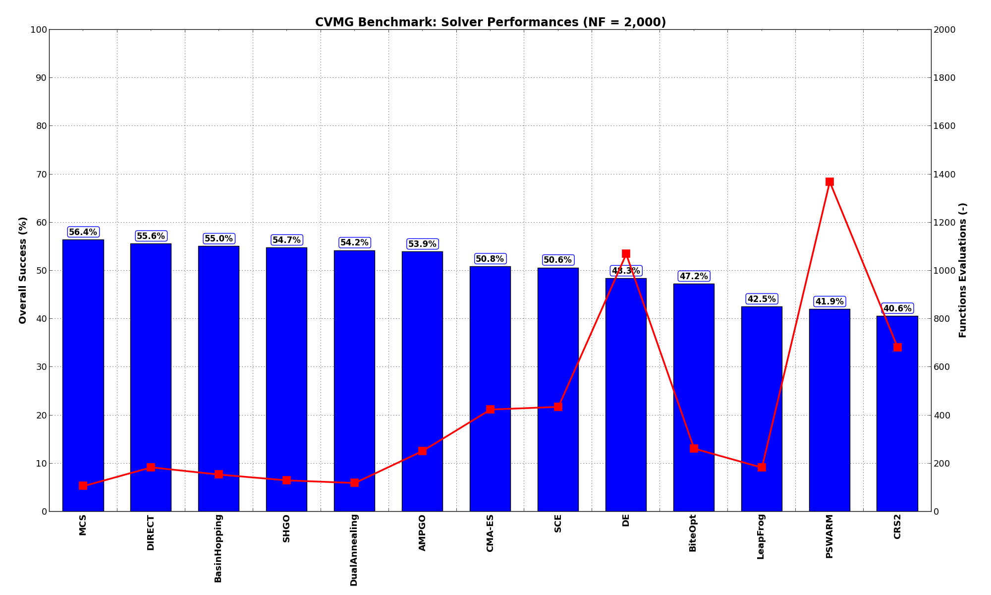
Optimization algorithms performances on the CVMG test suite at :math:`NF = 2,000`

Figure 13.2: Optimization algorithms performances on the CVMG test suite at $NF = 2,000$

Pushing the available budget to a very generous 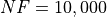$NF = 10,000$ , the results show AMPGO snatching the top spot from MCS, which is anyway very close to it in second place. As before, DIRECT, BasinHopping, SHGO and DualAnnealing are not that far behind. The results are also shown visually in Figure 13.3.

**Table 13.2**: Solvers performances on the CVMG benchmark suite at NF = 10,000
Optimization Method	Overall Success (%)	Functions Evaluations
AMPGO	58.33%	550
BasinHopping	55.83%	199
BiteOpt	49.17%	517
CMA-ES	53.33%	563
CRS2	40.56%	683
DE	53.06%	1,248
DIRECT	56.11%	223
DualAnnealing	54.72%	149
LeapFrog	42.50%	184
MCS	56.94%	155
PSWARM	48.89%	1,522
SCE	53.61%	669
SHGO	56.11%	245

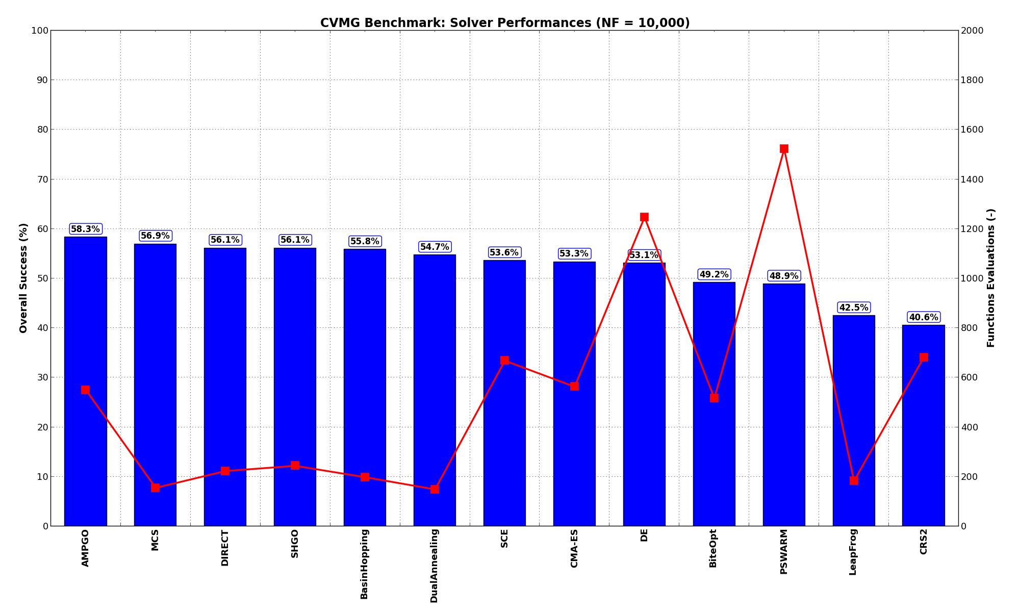
Optimization algorithms performances on the CVMG test suite at :math:`NF = 10,000`

Figure 13.3: Optimization algorithms performances on the CVMG test suite at $NF = 10,000$

Sensitivities on Functions Evaluations Budget¶

It is also interesting to analyze the success of an optimization algorithm based on the fraction (or percentage) of problems solved given a fixed number of allowed function evaluations, let’s say 100, 200, 300,... 2000, 5000, 10000.

In order to do that, we can present the results using two different types of visualizations. The first one is some sort of “small multiples” in which each solver gets an individual subplot showing the improvement in the number of solved problems as a function of the available number of function evaluations - on top of a background set of grey, semi-transparent lines showing all the other solvers performances.

This visual gives an indication of how good/bad is a solver compared to all the others as function of the budget available. Results are shown in Figure 13.4.

Figure 13.4: Percentage of problems solved given a fixed number of function evaluations on the CVMG test suite

The second type of visualization is sometimes referred as “Slopegraph” and there are many variants on the plot layout and appearance that we can implement. The version shown in Figure 13.5 aggregates all the solvers together, so it is easier to spot when a solver overtakes another or the overall performance of an algorithm while the available budget of function evaluations changes.

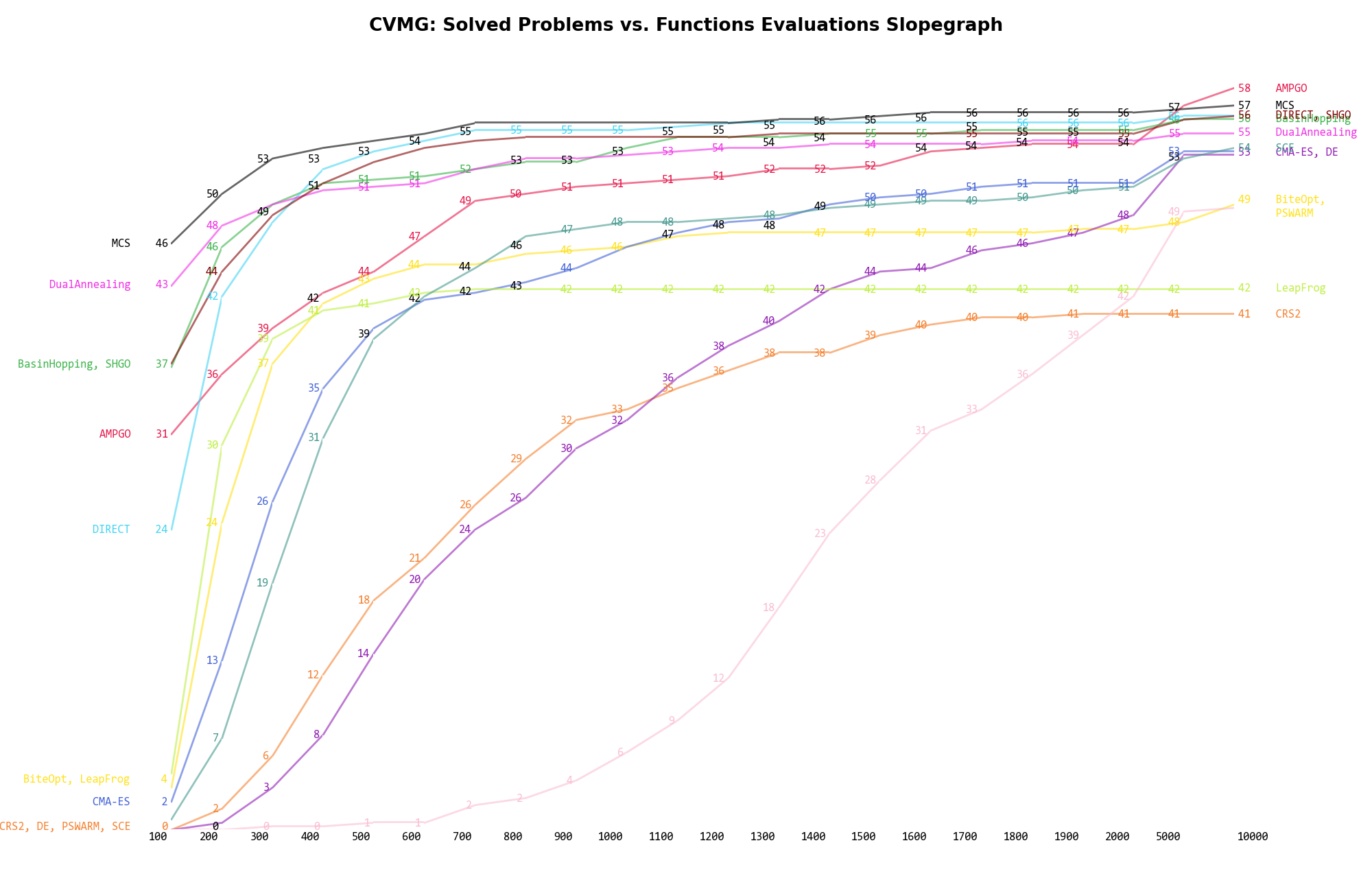
Figure 13.5: Percentage of problems solved given a fixed number of function evaluations on the CVMG test suite

A few obvious conclusions we can draw from these pictures are:

For this specific benchmark test suite, MCS is the best solver up to very large budgets of function evaluations. At the very end, AMPGO manages to gain first place but only for $NF = 10,000$ .
Quite a few other solvers display very good convergence results at lower budgets, namely DualAnnealing, SHGO and DIRECT.

Dimensionality Effects¶

Since I used the CVMG test suite to generate test functions with dimensionality ranging from 2 to 5, it is interesting to take a look at the solvers performances as a function of the problem dimensionality. Of course, in general it is to be expected that for larger dimensions less problems are going to be solved - although it is not always necessarily so as it also depends on the function being generated. Results are shown in Table 13.3 .

**Table 13.3**: Dimensionality effects on the CVMG benchmark suite at NF = 2,000
Solver	N = 2	N = 3	N = 4	N = 5	Overall
AMPGO	88.9	71.1	36.7	18.9	53.9
BasinHopping	91.1	75.6	34.4	18.9	55.0
BiteOpt	86.7	57.8	30.0	14.4	47.2
CMA-ES	88.9	67.8	28.9	17.8	50.8
CRS2	67.8	53.3	24.4	16.7	40.6
DE	88.9	73.3	28.9	2.2	48.3
DIRECT	91.1	76.7	36.7	17.8	55.6
DualAnnealing	91.1	72.2	34.4	18.9	54.2
LeapFrog	75.6	58.9	23.3	12.2	42.5
MCS	91.1	77.8	36.7	20.0	56.4
PSWARM	84.4	58.9	15.6	8.9	41.9
SCE	76.7	71.1	35.6	18.9	50.6
SHGO	91.1	76.7	36.7	14.4	54.7

Figure 13.6 shows the same results in a visual way.

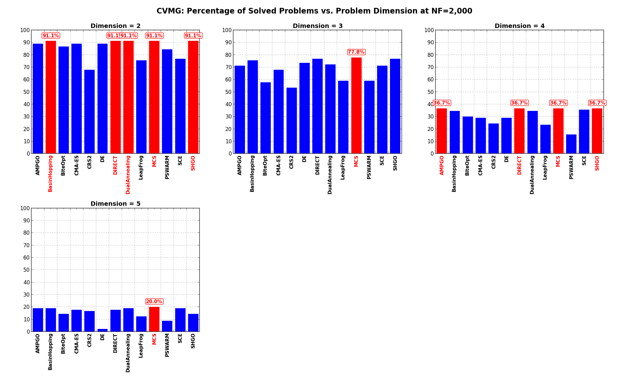
Percentage of problems solved as a function of problem dimension at :math:`NF = 2,000`

Figure 13.6: Percentage of problems solved as a function of problem dimension for the CVMG test suite at $NF = 2,000$

What we can infer from the table and the figure is that, for low dimensionality problems ( $NF = 2$ ), very many solvers are able to solve most of the problems in this test suite, with MCS, DIRECT, BasinHopping, SHGO and DualAnnealing leading the pack. By increasing the dimensionality those solvers stay close to one another but of course the percentage of solved problems decrease dramatically.

Pushing the available budget to a very generous $NF = 10,000$ shows AMPGO taking the lead for higher dimensional problems ( $N \geq 4$ ), finally coming up as the winner for this benchmark test suite.

The results for the benchmarks at $NF = 10,000$ are displayed in Table 13.4 and Figure 13.7.

**Table 13.4**: Dimensionality effects on the CVMG benchmark suite at NF = 10,000
Solver	N = 2	N = 3	N = 4	N = 5	Overall
AMPGO	91.1	77.8	41.1	23.3	58.3
BasinHopping	91.1	75.6	36.7	20.0	55.8
BiteOpt	88.9	63.3	30.0	14.4	49.2
CMA-ES	90.0	70.0	33.3	20.0	53.3
CRS2	67.8	53.3	24.4	16.7	40.6
DE	88.9	73.3	31.1	18.9	53.1
DIRECT	91.1	76.7	36.7	20.0	56.1
DualAnnealing	91.1	74.4	34.4	18.9	54.7
LeapFrog	75.6	58.9	23.3	12.2	42.5
MCS	91.1	77.8	37.8	21.1	56.9
PSWARM	85.6	64.4	26.7	18.9	48.9
SCE	87.8	71.1	35.6	20.0	53.6
SHGO	91.1	76.7	36.7	20.0	56.1

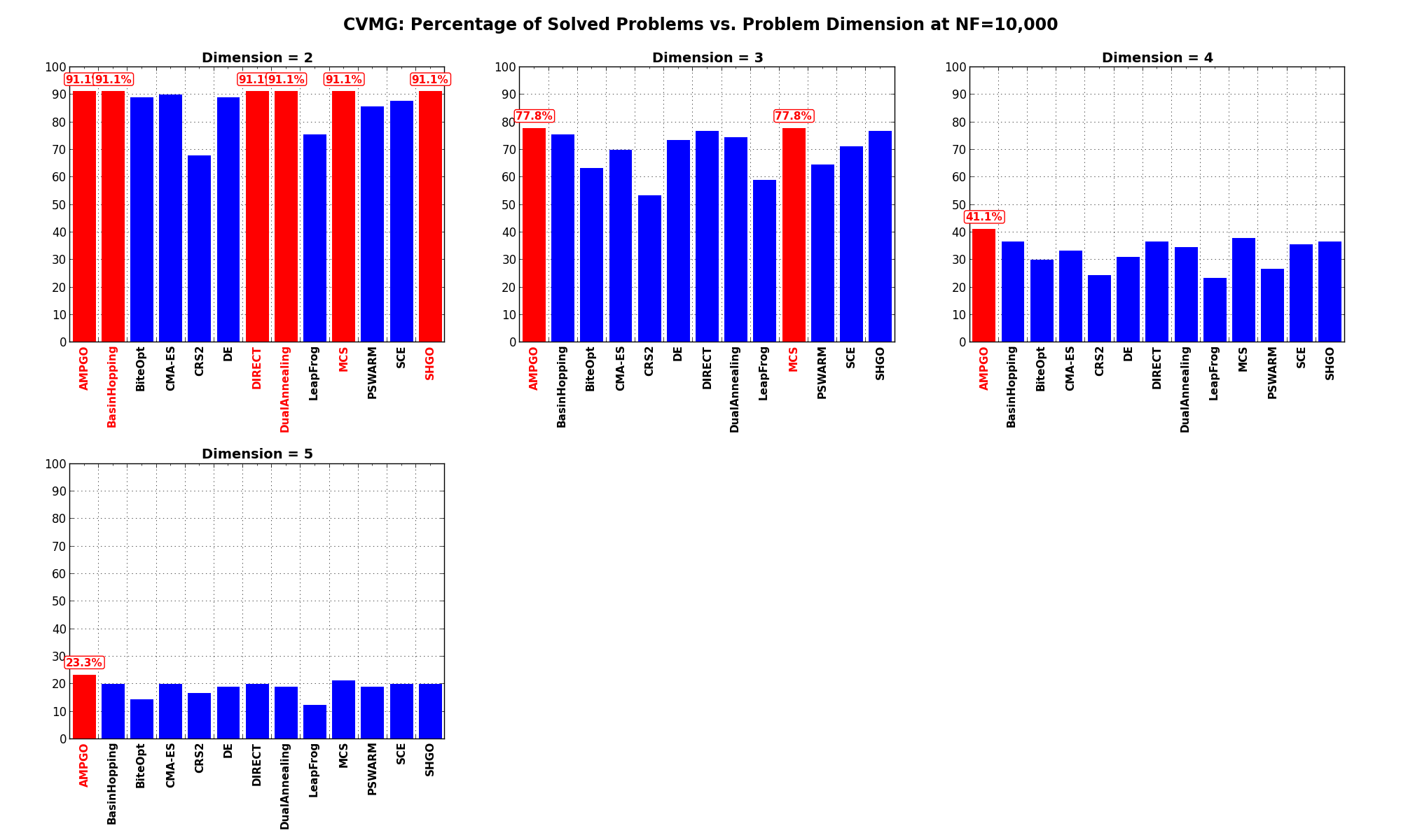
Percentage of problems solved as a function of problem dimension at :math:`NF = 10,000`

Figure 13.7: Percentage of problems solved as a function of problem dimension for the CVMG test suite at $NF = 10,000$

CVMG¶

Methodology¶

General Solvers Performances¶

Sensitivities on Functions Evaluations Budget¶

Dimensionality Effects¶

Table Of Contents

Previous topic

Next topic

This Page

Navigation

CVMG¶

Methodology¶

General Solvers Performances¶

Sensitivities on Functions Evaluations Budget¶

Dimensionality Effects¶

Table Of Contents

Previous topic

Next topic

This Page

Quick search

Navigation