Navigation
- index
- next |
- previous |

- Home »
- The Benchmarks »
- Robust
 Robust
| Fopt Known | Xopt Known | Difficulty |
|---|---|---|
| Yes | Yes | Medium |
This is the last benchmark of the series, and you will forgive me if I stop after this... The Robust test suite is actually composed of 5 different kind-of analytical test function generators, containing deceptive, multimodal, flat functions depending on the settings. The theory behind this test suite is described in the paper https://www.sciencedirect.com/science/article/pii/S0020025515006301 . Matlab source code is available at http://www.alimirjalili.com/RO.html , I simply converted it to Python.
 Methodology
The actual objective functions created by this test function generator depend on which generator is actually chosen - 5 of them are available.
For generator I:
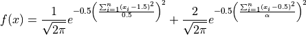
Where  indicates the robustness of the global optimum by narrowing or widening it. The robustness of the global optimum is
decreased proportionally to the value of the parameter .
indicates the robustness of the global optimum by narrowing or widening it. The robustness of the global optimum is
decreased proportionally to the value of the parameter .
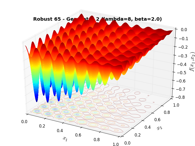
For generator II:

Where:
![H(x) = \frac{e^{-2x^2} \sin \left [ 2 \pi \lambda \left (x + \frac{\pi}{4 \lambda} \right ) \right ] - x^{\beta}} {3} + 0.5](_images/math/56f21be56068c4491fc7a36327bb402f2f9e778e.png)
This benchmark generator allows generating  number of local optima through the search space. The search space becomes
more challenging as
number of local optima through the search space. The search space becomes
more challenging as  increases.
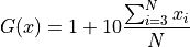
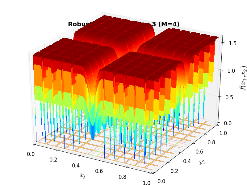
For generator III:

Where:

This benchmark generator generates deceptive test functions.
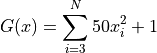
For generator IV:

Where:

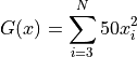
This benchmark generator generates flat test functions.
For the Robust benchmark, I have created 420 test functions with dimensionality ranging from 2 to 6.
A few examples of 2D benchmark functions created with the Robust generator can be seen in Figure 16.1.

Robust Function 2 |
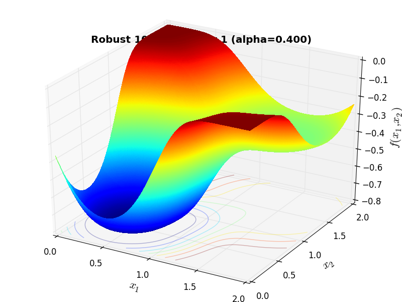
Robust Function 10 |
Robust Function 65 |
Robust Function 173 |
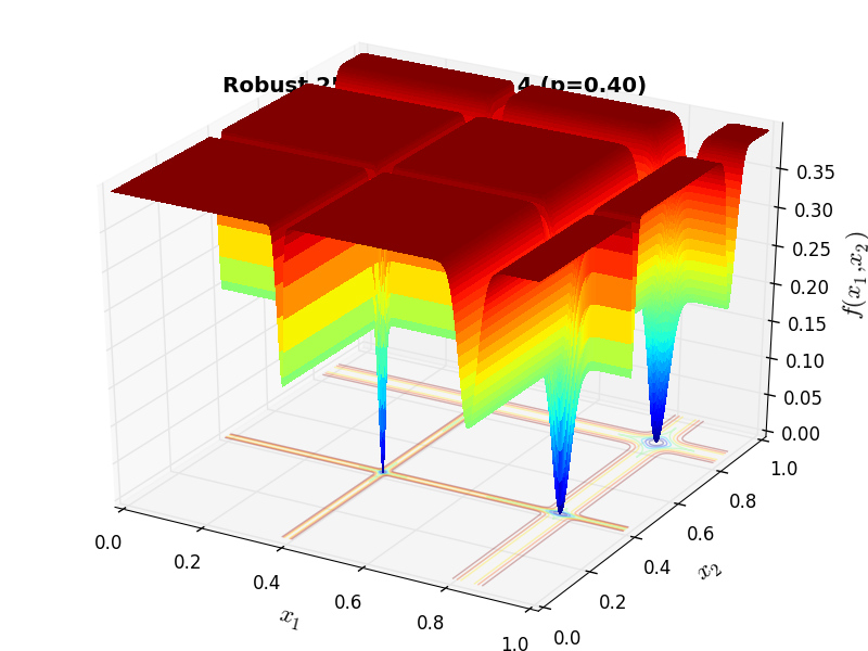
Robust Function 253 |
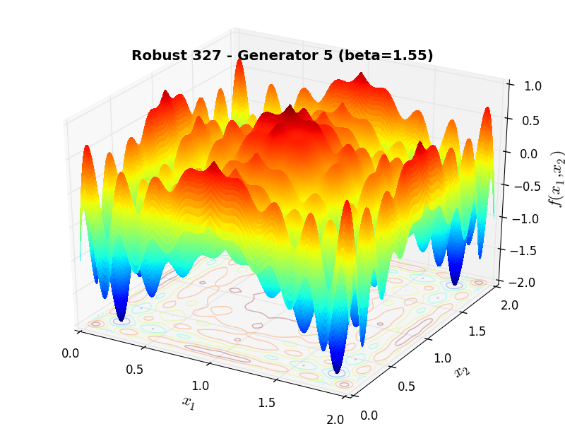
Robust Function 327 |
 General Solvers Performances
Table 16.1 below shows the overall success of all Global Optimization algorithms, considering every benchmark function,
for a maximum allowable budget of  .
.
The Robust benchmark suite is a medium-difficulty test suite: the best solver for is BiteOpt, with a success
rate of 62.4%, followed at a distance by AMPGO and DualAnnealing.
Note
The reported number of functions evaluations refers to successful optimizations only.
| Optimization Method | Overall Success (%) | Functions Evaluations |
|---|---|---|
| AMPGO | 52.14% | 583 |
| BasinHopping | 36.19% | 651 |
| BiteOpt | 62.38% | 383 |
| CMA-ES | 33.57% | 768 |
| CRS2 | 40.48% | 892 |
| DE | 27.86% | 1,146 |
| DIRECT | 45.71% | 600 |
| DualAnnealing | 51.43% | 569 |
| LeapFrog | 22.86% | 177 |
| MCS | 45.48% | 268 |
| PSWARM | 28.10% | 1,457 |
| SCE | 23.10% | 710 |
| SHGO | 36.43% | 368 |
These results are also depicted in Figure 16.2, which shows that BiteOpt is the better-performing optimization algorithm, followed at a distance by AMPGO and DualAnnealing.
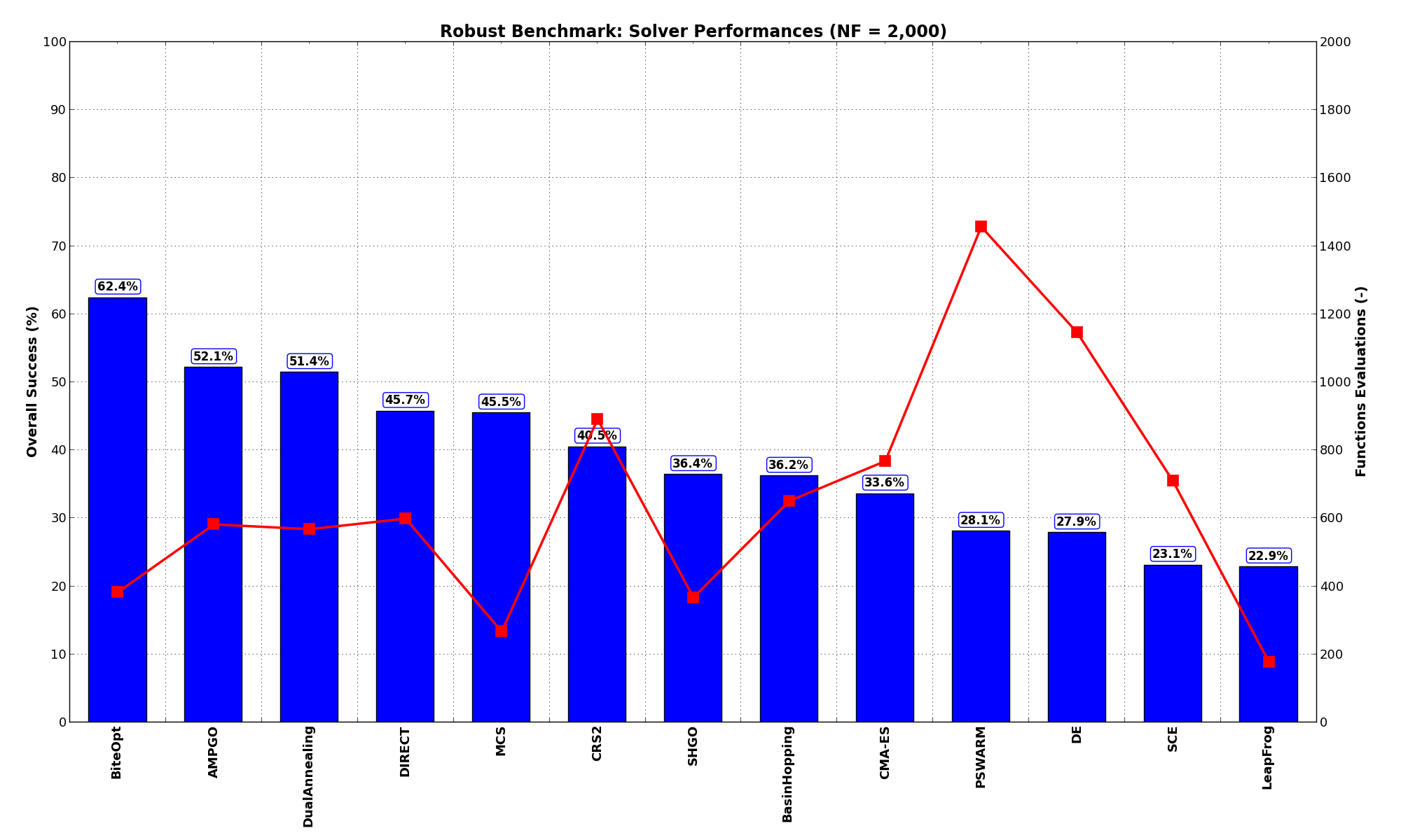
Figure 16.2: Optimization algorithms performances on the Robust test suite at
Pushing the available budget to a very generous  , the results show AMPGO snatching the top spot from BiteOpt,
although the two algorithms are close. DualAnnealing and MCS trail behind at a large distance.
The results are also shown visually in Figure 16.3.
, the results show AMPGO snatching the top spot from BiteOpt,
although the two algorithms are close. DualAnnealing and MCS trail behind at a large distance.
The results are also shown visually in Figure 16.3.
| Optimization Method | Overall Success (%) | Functions Evaluations |
|---|---|---|
| AMPGO | 75.95% | 1,897 |
| BasinHopping | 41.67% | 1,100 |
| BiteOpt | 73.10% | 1,272 |
| CMA-ES | 58.10% | 2,330 |
| CRS2 | 51.43% | 1,463 |
| DE | 59.05% | 3,614 |
| DIRECT | 49.05% | 771 |
| DualAnnealing | 64.76% | 1,317 |
| LeapFrog | 23.81% | 182 |
| MCS | 59.52% | 1,268 |
| PSWARM | 51.19% | 1,967 |
| SCE | 31.19% | 1,726 |
| SHGO | 44.29% | 1,630 |
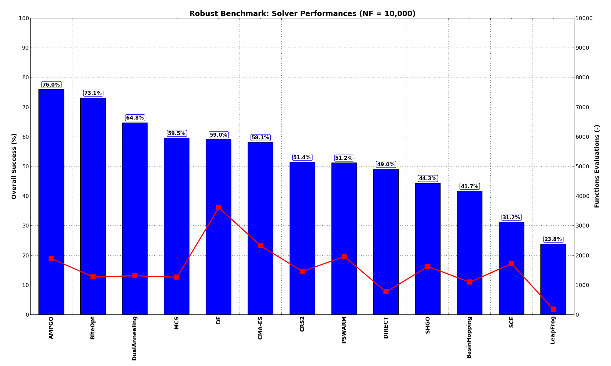
Figure 16.3: Optimization algorithms performances on the Robust test suite at
 Sensitivities on Functions Evaluations Budget
It is also interesting to analyze the success of an optimization algorithm based on the fraction (or percentage) of problems solved given a fixed number of allowed function evaluations, let’s say 100, 200, 300,... 2000, 5000, 10000.
In order to do that, we can present the results using two different types of visualizations. The first one is some sort of “small multiples” in which each solver gets an individual subplot showing the improvement in the number of solved problems as a function of the available number of function evaluations - on top of a background set of grey, semi-transparent lines showing all the other solvers performances.
This visual gives an indication of how good/bad is a solver compared to all the others as function of the budget available. Results are shown in Figure 16.4.
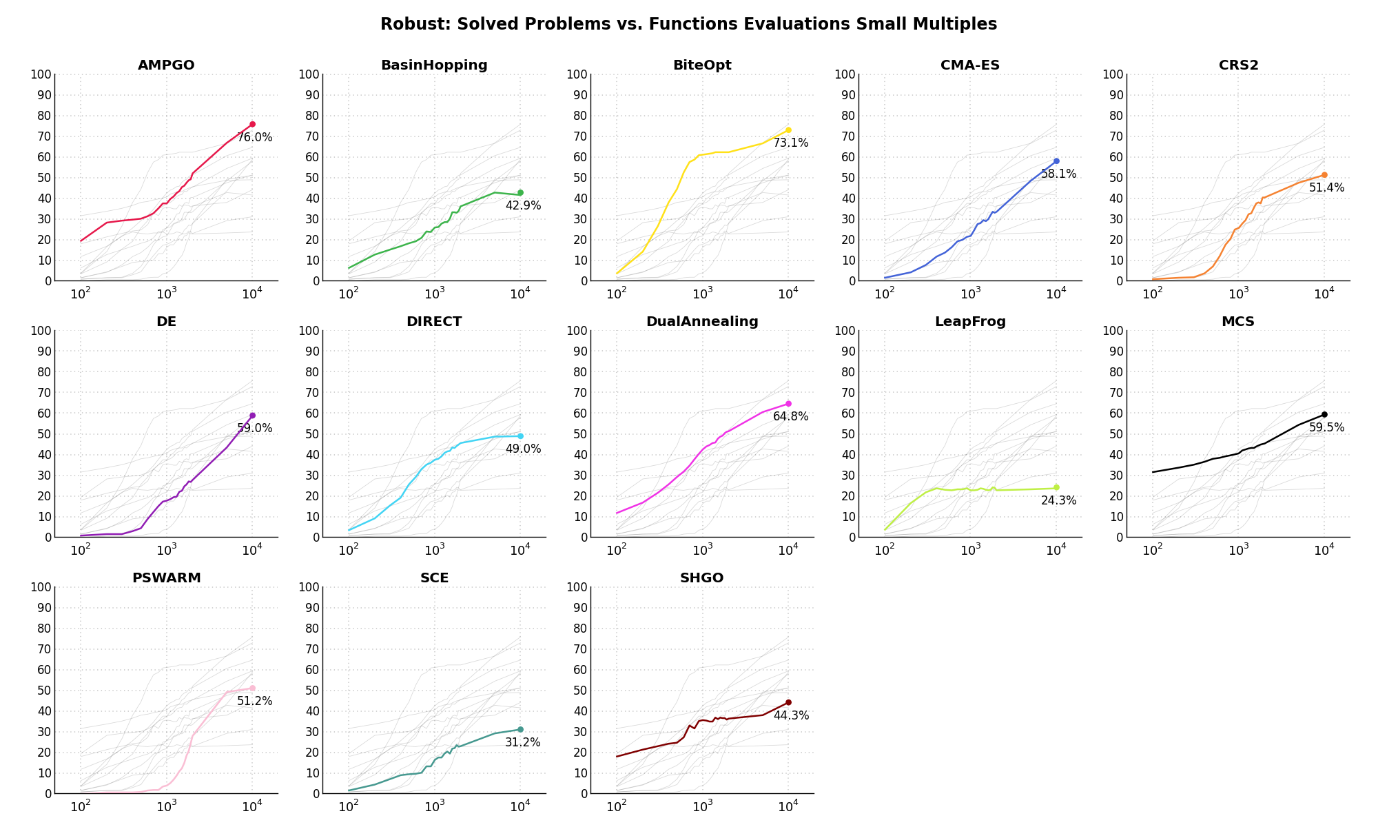
Figure 16.4: Percentage of problems solved given a fixed number of function evaluations on the Robust test suite
The second type of visualization is sometimes referred as “Slopegraph” and there are many variants on the plot layout and appearance that we can implement. The version shown in Figure 16.5 aggregates all the solvers together, so it is easier to spot when a solver overtakes another or the overall performance of an algorithm while the available budget of function evaluations changes.
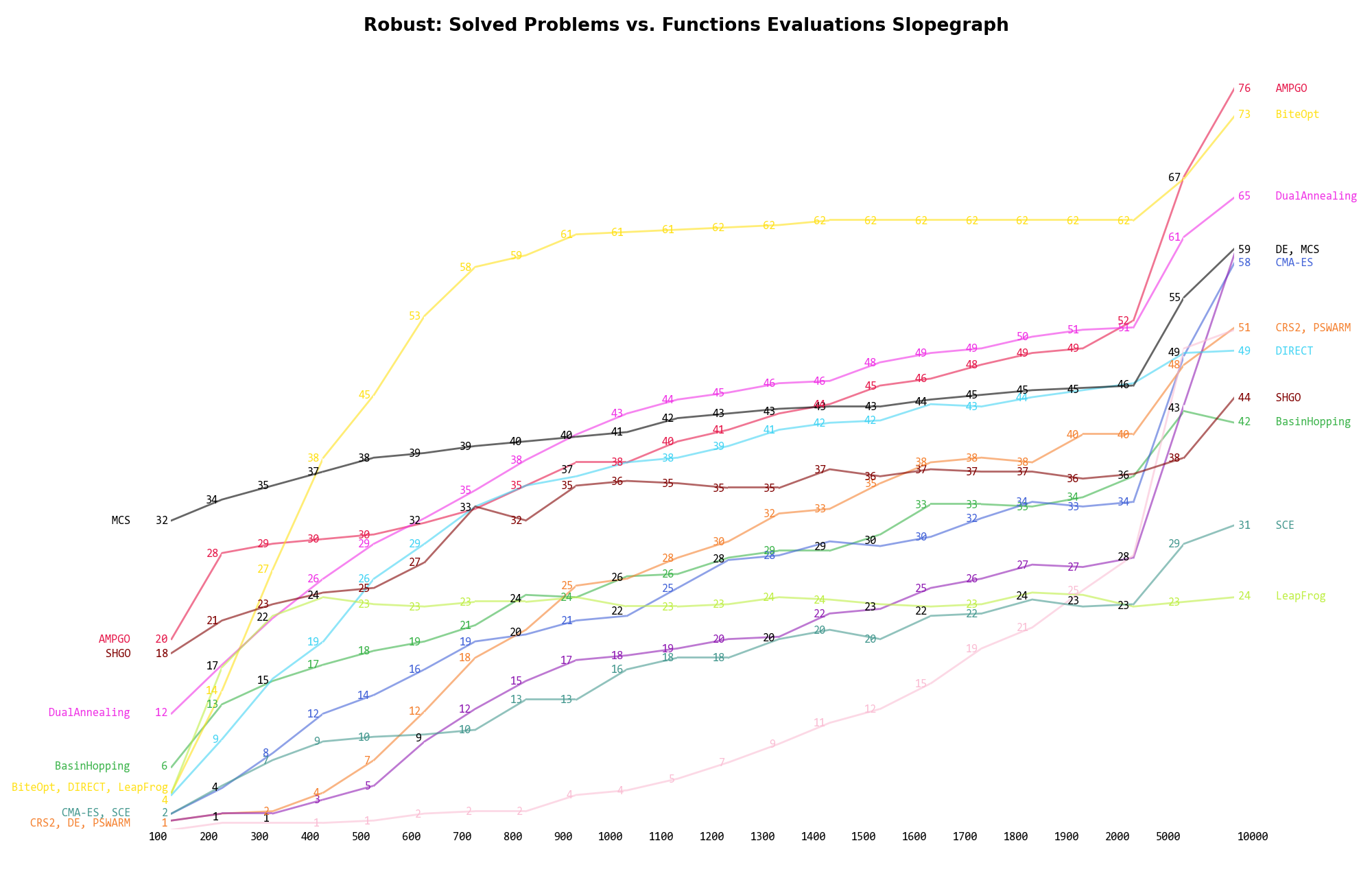
Figure 16.5: Percentage of problems solved given a fixed number of function evaluations on the Robust test suite
A few obvious conclusions we can draw from these pictures are:
 ) MCS appears to be
the most successful solver.
) MCS appears to be
the most successful solver. Dimensionality Effects
Since I used the Robust test suite to generate test functions with dimensionality ranging from 2 to 6, it is interesting to take a look at the solvers performances as a function of the problem dimensionality. Of course, in general it is to be expected that for larger dimensions less problems are going to be solved - although it is not always necessarily so as it also depends on the function being generated. Results are shown in Table 16.3 .
| Solver | N = 2 | N = 3 | N = 4 | N = 5 | N = 6 | Overall |
|---|---|---|---|---|---|---|
| AMPGO | 72.6 | 57.1 | 45.2 | 48.8 | 36.9 | 52.1 |
| BasinHopping | 58.3 | 40.5 | 34.5 | 23.8 | 23.8 | 36.2 |
| BiteOpt | 91.7 | 54.8 | 57.1 | 54.8 | 53.6 | 62.4 |
| CMA-ES | 56.0 | 46.4 | 29.8 | 23.8 | 11.9 | 33.6 |
| CRS2 | 63.1 | 52.4 | 40.5 | 32.1 | 14.3 | 40.5 |
| DE | 81.0 | 46.4 | 8.3 | 3.6 | 0.0 | 27.9 |
| DIRECT | 71.4 | 51.2 | 50.0 | 44.0 | 11.9 | 45.7 |
| DualAnnealing | 79.8 | 50.0 | 52.4 | 40.5 | 34.5 | 51.4 |
| LeapFrog | 45.2 | 27.4 | 10.7 | 15.5 | 15.5 | 22.9 |
| MCS | 67.9 | 59.5 | 35.7 | 33.3 | 31.0 | 45.5 |
| PSWARM | 48.8 | 28.6 | 28.6 | 19.0 | 15.5 | 28.1 |
| SCE | 59.5 | 31.0 | 21.4 | 3.6 | 0.0 | 23.1 |
| SHGO | 89.3 | 28.6 | 27.4 | 17.9 | 19.0 | 36.4 |
Figure 16.6 shows the same results in a visual way.
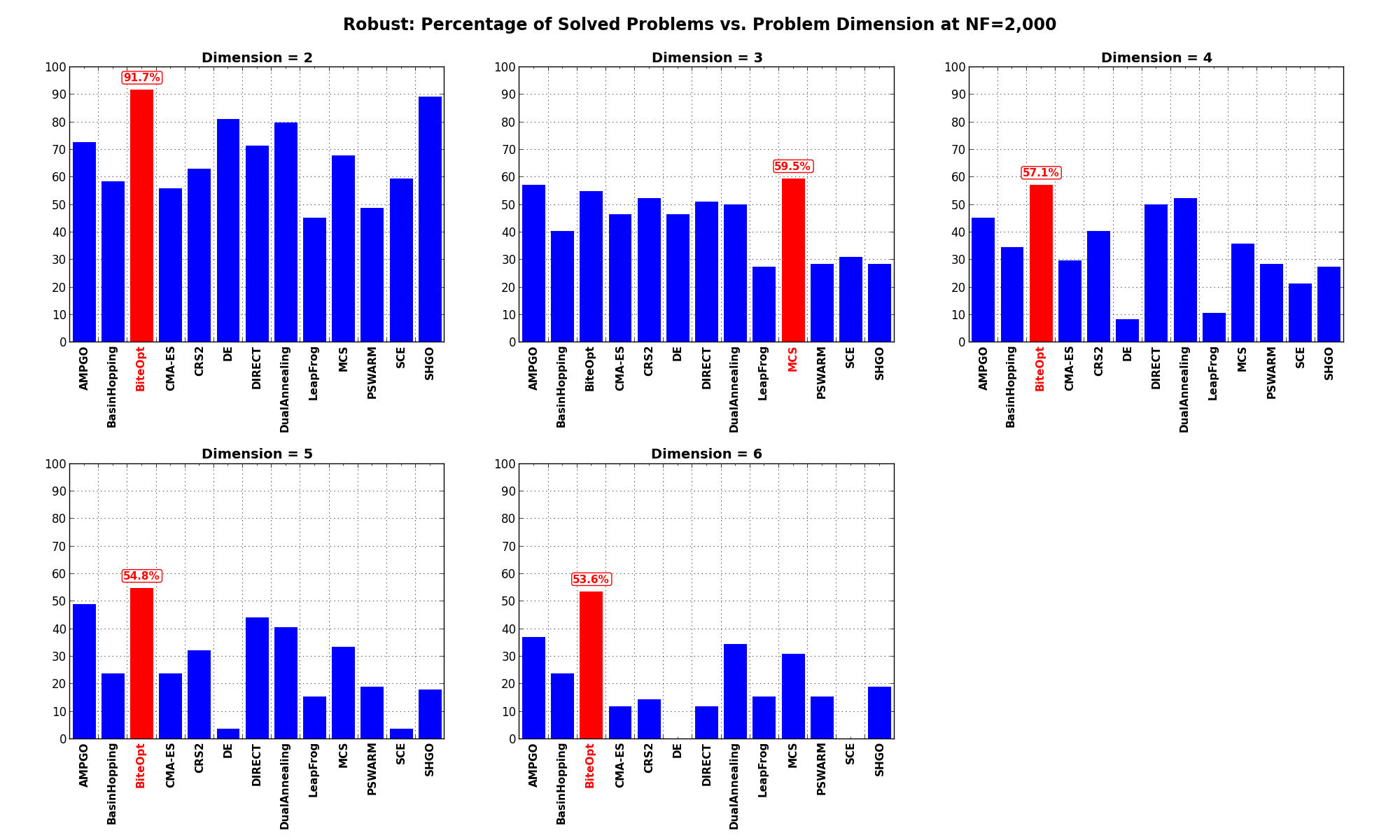
Figure 16.6: Percentage of problems solved as a function of problem dimension for the Robust test suite at
What we can infer from the table and the figure is that, for pretty much all dimensionalities, BiteOpt displays much
better convergence rates than other solvers, only slightly beaten for  by MCS.
Pushing the available budget to a very generous shows SHGO scoring a perfect 100% success rate for
low dimensionality problems ( ) while AMPGO shows extremely high rates of success for higher dimensionalities.
The results for the benchmarks at are displayed in Table 16.4 and Figure 16.7.
| Solver | N = 2 | N = 3 | N = 4 | N = 5 | N = 6 | Overall |
|---|---|---|---|---|---|---|
| AMPGO | 86.9 | 82.1 | 75.0 | 69.0 | 66.7 | 76.0 |
| BasinHopping | 63.1 | 39.3 | 48.8 | 29.8 | 27.4 | 41.7 |
| BiteOpt | 94.0 | 72.6 | 81.0 | 61.9 | 56.0 | 73.1 |
| CMA-ES | 64.3 | 63.1 | 60.7 | 52.4 | 50.0 | 58.1 |
| CRS2 | 61.9 | 56.0 | 58.3 | 46.4 | 34.5 | 51.4 |
| DE | 83.3 | 81.0 | 54.8 | 46.4 | 29.8 | 59.0 |
| DIRECT | 72.6 | 51.2 | 50.0 | 48.8 | 22.6 | 49.0 |
| DualAnnealing | 85.7 | 61.9 | 63.1 | 59.5 | 53.6 | 64.8 |
| LeapFrog | 48.8 | 27.4 | 10.7 | 16.7 | 15.5 | 23.8 |
| MCS | 85.7 | 79.8 | 51.2 | 41.7 | 39.3 | 59.5 |
| PSWARM | 70.2 | 66.7 | 59.5 | 33.3 | 26.2 | 51.2 |
| SCE | 69.0 | 41.7 | 39.3 | 4.8 | 1.2 | 31.2 |
| SHGO | 100.0 | 53.6 | 21.4 | 25.0 | 21.4 | 44.3 |
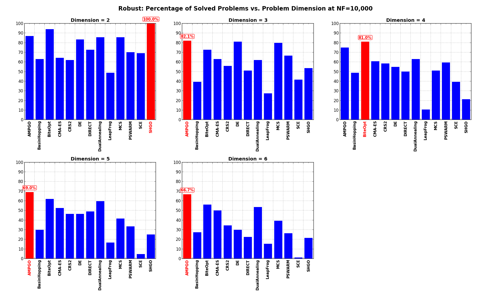
Figure 16.7: Percentage of problems solved as a function of problem dimension for the Robust test suite at