NIST¶

F_opt Known	X_opt Known	Difficulty
Yes	Yes	Medium

This benchamrk test suite is not exactly the realm of Global Optimization solvers, but the NIST StRD dataset can be used to generate a single objective function as “sum of squares”. I have used the NIST dataset as implemented in lmfit.

The NIST datasets are ordered by level of difficulty (lower, average, and higher). This ordering is meant to provide rough guidance for the user. Producing correct results on all datasets of higher difficulty does not imply that the solver will correctly solve all datasets of average or even lower difficulty. Similarly, producing correct results for all datasets in this collection does not imply that your optimization algorithm will do the same for your own particular dataset. It will, however, provide some degree of assurance, in the sense that a specific solver provides correct results for datasets known to yield incorrect results for some software.

The robustness and reliability of nonlinear least squares solvers depends on the algorithm used and how it is implemented, as well as on the characteristics of the actual problem being solved. Nonlinear least squares solvers are particularly sensitive to the starting values provided for a given problem. For this reason, NIST provides three sets of starting values for each problem: the first is relatively far from the final solution; the second relatively close; and the third is the actual certified solution.

In this specific instance, for solvers that accepts an initial starting point $x_0$ , I have provided them with the first one specified by NIST. For algorithms which do not accept a starting point, tough luck: life isn’t fair.

Note

NIST does not provide bounds on the parameters for its models, but by examining the two starting points and the certified solutions provided by NIST it is possible to build a set of very loose bounds for the optimization variables.

Methodology¶

There isn’t much to describe in terms of methodology, as the equations, data, starting points, certified solutions and level of difficulty have been clearly spelled out by NIST. Table 11.1 below gives an overview of the various problems in terms of dimensionality, the equations and level of difficulty.

**Table 11.1**: NIST dataset summary
Name	Dimension	Difficulty	Function
Bennett5	3	Higher	$y = \beta_{1} \left(\beta_{2} + x\right)^{- 1 / \beta_{3}}$
BoxBOD	2	Higher	$y = \beta_{1} \left(1 - e^{- \beta_{2} x}\right)$
Chwirut1	3	Lower	$y = \frac{e^{- \beta_{1} x}}{\beta_{2} + \beta_{3} x}$
Chwirut2	3	Lower	$y = \frac{e^{- \beta_{1} x}}{\beta_{2} + \beta_{3} x}$
DanWood	2	Lower	$y = \beta_{1} x^{\beta_{2}}$
ENSO	9	Average	$y = \beta_{1} + \beta_{2} \cos{\left (\pi x / 6 \right )} + \beta_{3} \sin{\left (\pi x / 6 \right )} + \beta_{5} \cos{\left (2 \pi x / \beta_{4} \right )} + \beta_{6} \sin{\left (2 \pi x / \beta_{4} \right )} + \beta_{8} \cos{\left (2 \pi x / \beta_{7} \right )} + \beta_{9} \sin{\left (2 \pi x / \beta_{7} \right )}$
Eckerle4	3	Higher	$y = \beta_{1} e^{- \frac{0.5}{\beta_{2}^{2}} \left(- \beta_{3} + x\right)^{2}} / \beta_{2}$
Gauss1	8	Lower	$y = \beta_{1} e^{- \beta_{2} x} + \beta_{3} e^{- \frac{1}{\beta_{5}^{2}} \left(- \beta_{4} + x\right)^{2}} + \beta_{6} e^{- \frac{1}{\beta_{8}^{2}} \left(- \beta_{7} + x\right)^{2}}$
Gauss2	8	Lower	$y = \beta_{1} e^{- \beta_{2} x} + \beta_{3} e^{- \frac{1}{\beta_{5}^{2}} \left(- \beta_{4} + x\right)^{2}} + \beta_{6} e^{- \frac{1}{\beta_{8}^{2}} \left(- \beta_{7} + x\right)^{2}}$
Gauss3	8	Average	$y = \beta_{1} e^{- \beta_{2} x} + \beta_{3} e^{- \frac{1}{\beta_{5}^{2}} \left(- \beta_{4} + x\right)^{2}} + \beta_{6} e^{- \frac{1}{\beta_{8}^{2}} \left(- \beta_{7} + x\right)^{2}}$
Hahn1	7	Average	$y = \frac{\beta_{1} + \beta_{2} x + \beta_{3} x^{2} + \beta_{4} x^{3}}{\beta_{5} x + \beta_{6} x^{2} + \beta_{7} x^{3} + 1}$
Kirby2	5	Average	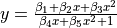$y = \frac{\beta_{1} + \beta_{2} x + \beta_{3} x^{2}}{\beta_{4} x + \beta_{5} x^{2} + 1}$
Lanczos1	6	Average	$y = \beta_{1} e^{- \beta_{2} x} + \beta_{3} e^{- \beta_{4} x} + \beta_{5} e^{- \beta_{6} x}$
Lanczos2	6	Average	$y = \beta_{1} e^{- \beta_{2} x} + \beta_{3} e^{- \beta_{4} x} + \beta_{5} e^{- \beta_{6} x}$
Lanczos3	6	Lower	$y = \beta_{1} e^{- \beta_{2} x} + \beta_{3} e^{- \beta_{4} x} + \beta_{5} e^{- \beta_{6} x}$
MGH09	4	Higher	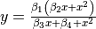$y = \frac{\beta_{1} \left(\beta_{2} x + x^{2}\right)}{\beta_{3} x + \beta_{4} + x^{2}}$
MGH10	3	Higher	$y = \beta_{1} e^{\frac{\beta_{2}}{\beta_{3} + x}}$
MGH17	5	Average	$y = \beta_{1} + \beta_{2} e^{- \beta_{4} x} + \beta_{3} e^{- \beta_{5} x}$
Misra1a	2	Lower	$y = \beta_{1} \left(1 - e^{- \beta_{2} x}\right)$
Misra1b	2	Lower	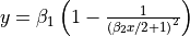$y = \beta_{1} \left(1 - \frac{1}{\left(\beta_{2} x / 2 + 1\right)^{2}}\right)$
Misra1c	2	Average	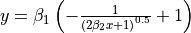$y = \beta_{1} \left(- \frac{1}{\left(2 \beta_{2} x + 1\right)^{0.5}} + 1\right)$
Misra1d	2	Average	$y = \frac{\beta_{1} \beta_{2} x}{\beta_{2} x + 1}$
Nelson	3	Average	$y = \beta_{1} - \beta_{2} x_{1} e^{- \beta_{3} x_{2}}$
Rat42	3	Higher	$y = \frac{\beta_{1}}{e^{\beta_{2} - \beta_{3} x} + 1}$
Rat43	4	Higher	$y = \beta_{1} \left(e^{\beta_{2} - \beta_{3} x} + 1\right)^{- 1.0 / \beta_{4}}$
Roszman1	4	Average	$y = \beta_{1} - \beta_{2} x - \arctan{\left (\frac{\beta_{3}}{- \beta_{4} + x} \right )} / \pi$
Thurber	7	Higher	$y = \frac{\beta_{1} + \beta_{2} x + \beta_{3} x^{2} + \beta_{4} x^{3}}{\beta_{5} x + \beta_{6} x^{2} + \beta_{7} x^{3} + 1}$

General Solvers Performances¶

Table 11.2 below shows the overall success of all Global Optimization algorithms, considering every benchmark function, for a maximum allowable budget of $NF = 2,000$ .

The NIST benchmark suite is a medium-difficulty test suite: the best solver for $NF = 2,000$ is MCS, with a success rate of 63.0%, followed by BiteOpt at a significant distance.

Note

The reported number of functions evaluations refers to successful optimizations only.

**Table 11.2**: Solvers performances on the NIST benchmark suite at NF = 2,000
Optimization Method	Overall Success (%)	Functions Evaluations
AMPGO	33.33%	383
BasinHopping	11.11%	230
BiteOpt	48.15%	1,091
CMA-ES	14.81%	940
CRS2	25.93%	1,314
DE	7.41%	1,320
DIRECT	3.70%	515
DualAnnealing	11.11%	308
LeapFrog	18.52%	681
MCS	62.96%	302
PSWARM	0.00%	0
SCE	29.63%	980
SHGO	7.41%	202

These results are also depicted in Figure 11.1, which shows that MCS is the better-performing optimization algorithm, followed by BiteOpt and AMPGO. Note that PSWARM has a 0% success rate i this case.

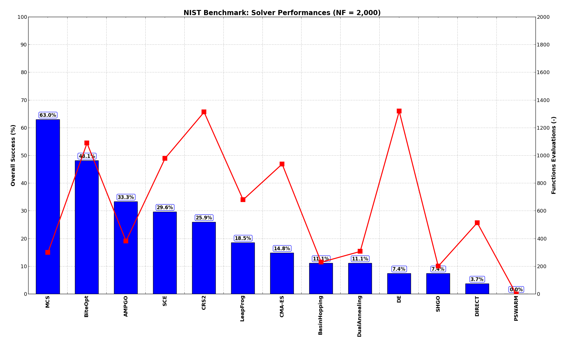
Optimization algorithms performances on the NIST test suite at :math:`NF = 2,000`

Figure 11.1: Optimization algorithms performances on the NIST test suite at $NF = 2,000$

Pushing the available budget to a very generous 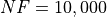$NF = 10,000$ , the results show MCS still keeping the lead, solving abot 74% of the problems, with BiteOpt and CRS2 tied at second place. The results are also shown visually in Figure 11.2.

**Table 11.3**: Solvers performances on the NIST benchmark suite at NF = 10,000
Optimization Method	Overall Success (%)	Functions Evaluations
AMPGO	51.85%	1,725
BasinHopping	14.81%	1,405
BiteOpt	70.37%	2,136
CMA-ES	44.44%	4,392
CRS2	70.37%	4,242
DE	40.74%	3,723
DIRECT	3.70%	515
DualAnnealing	14.81%	937
LeapFrog	22.22%	1,667
MCS	74.07%	630
PSWARM	7.41%	3,292
SCE	37.04%	1,423
SHGO	7.41%	202

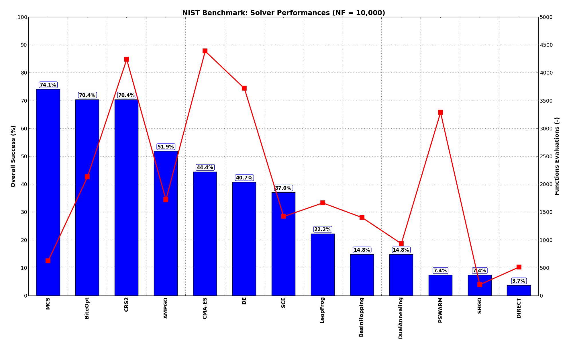
Optimization algorithms performances on the NIST test suite at :math:`NF = 10,000`

Figure 11.2: Optimization algorithms performances on the NIST test suite at $NF = 10,000$

In this specific test suite, it’s also interesting to show the actual outcome of the fit for some selected objective functions, and this is presented in Figure 11.3. a few remarks on these plots:

Red dots represent data points, while solid blue lines are the result of the fit coming from the best combination of parameters for each solver.
Each subplot holds a plot for a specific solver: if the title of a specific subplot is yellow, then convergence was not satisfactory (as highlighted by the $\Delta F$ label in the text inset).
Values for $R^2$ are also displayed in the text inset.

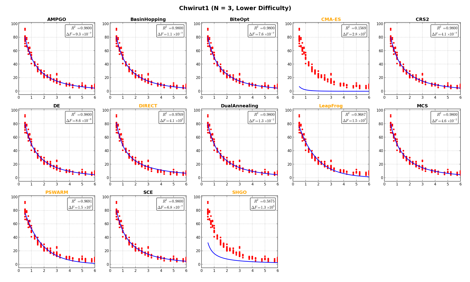
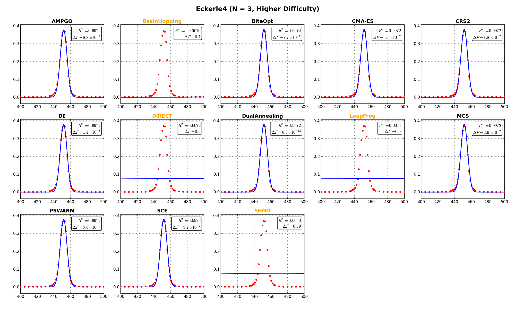
NIST Function Chwirut1	NIST Function Eckerle4
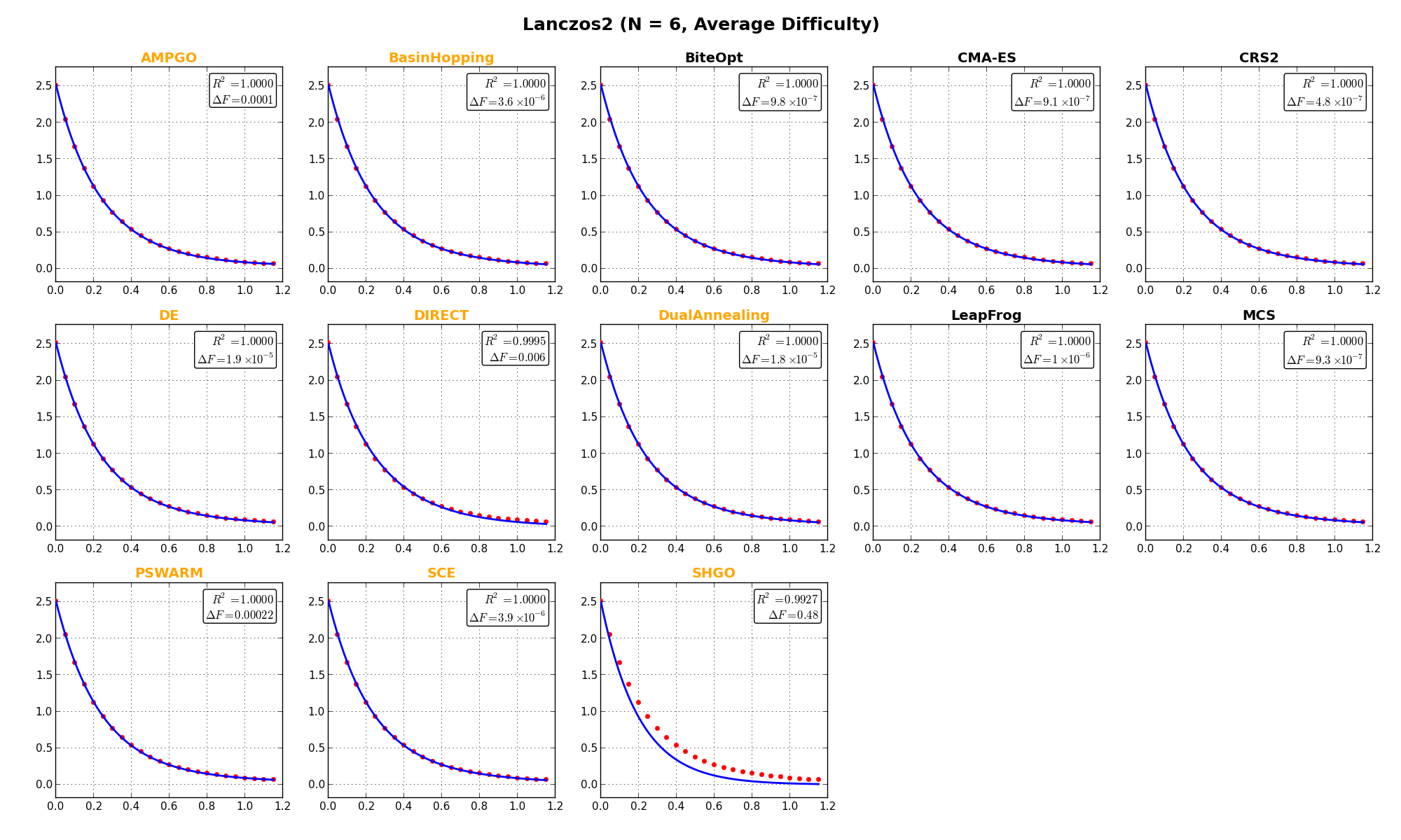
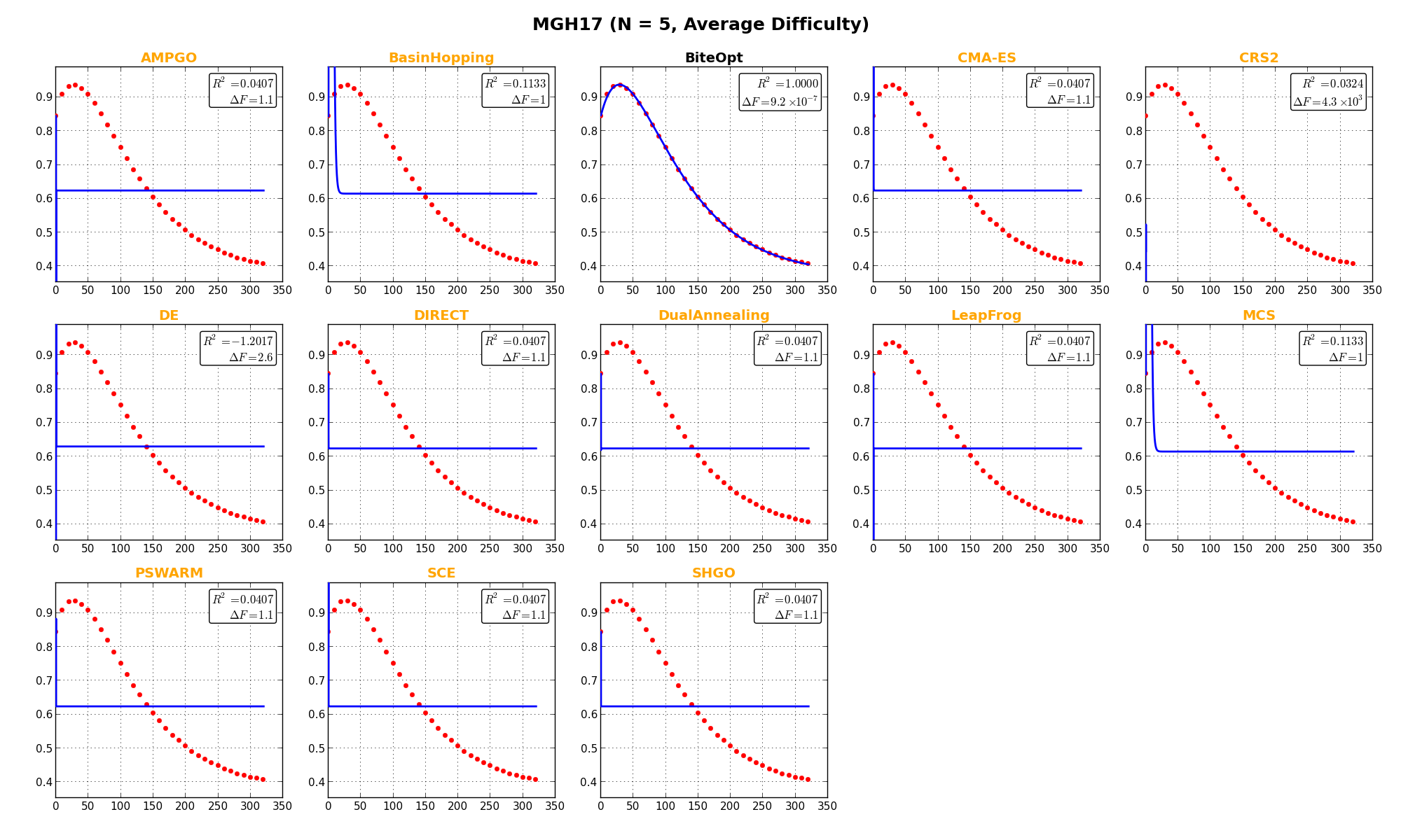
NIST Function Lanczos2	NIST Function MGH17
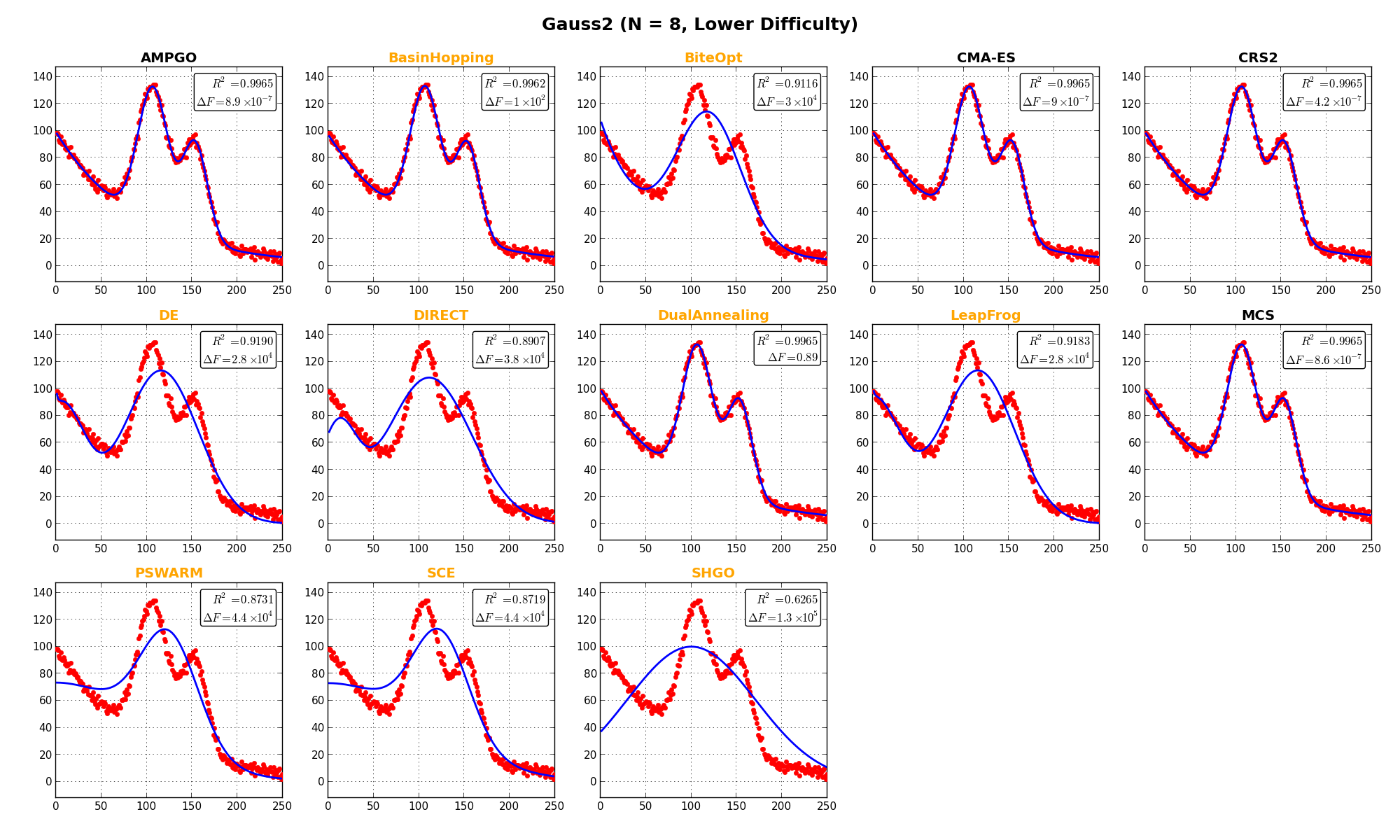
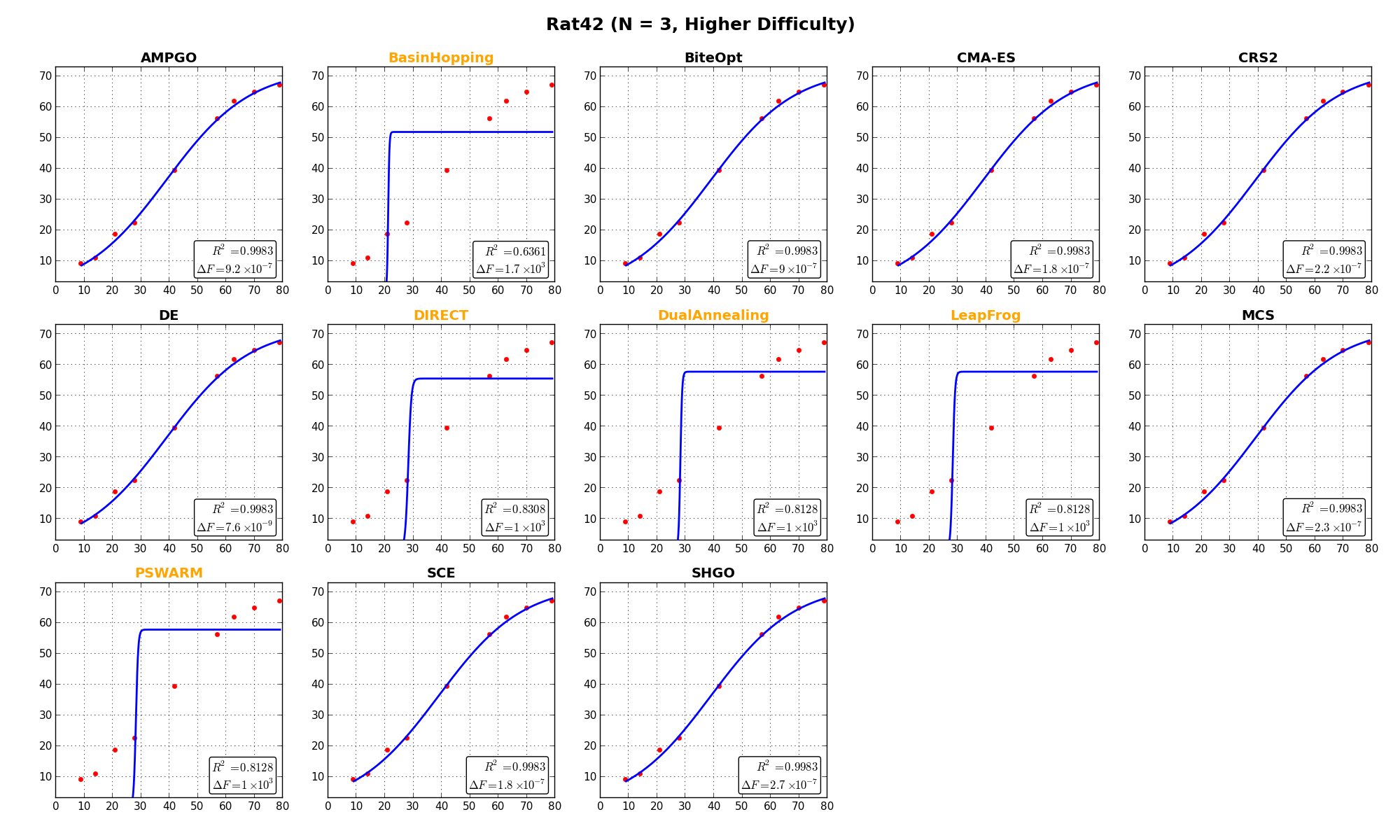
NIST Function Gauss2	NIST Function Rat42

It is also interesting to check whether there are instances of problems that are never solved, no matter the optimization algorithm. This is presented in Table 11.4 below. The table is not sorted by name this time, but in order of actual “difficulty” our solvers encountered in minimizing the NIST objective functions.

**Table 11.4**: Solvers performances on the NIST benchmark suite at NF = 10,000
Problem	AMPGO	BasinHopping	BiteOpt	CMA-ES	CRS2	DE	DIRECT	DualAnnealing	LeapFrog	MCS	PSWARM	SCE	SHGO
DanWood
Eckerle4
BoxBOD
Chwirut1
Rat42
Chwirut2
Misra1b
Misra1c
Misra1d
Roszman1
Gauss1
Lanczos2
ENSO
Gauss2
Lanczos1
Lanczos3
Gauss3
Kirby2
MGH09
Misra1a
Bennett5
MGH17
Nelson
Rat43
Thurber
Hahn1
MGH10

As can be seen, one NIST model was solved by all optimization algorithms (DanWood), while there were at least 2 solvers able to minimize correctly more than 20 functions. It has to be noted, for two of the NIST models no solvers were able to find any suitable set of parameters to satisfy convergence criteria (Hahn1 and MGH10).

Sensitivities on Functions Evaluations Budget¶

It is also interesting to analyze the success of an optimization algorithm based on the fraction (or percentage) of problems solved given a fixed number of allowed function evaluations, let’s say 100, 200, 300,... 2000, 5000, 10000.

In order to do that, we can present the results using two different types of visualizations. The first one is some sort of “small multiples” in which each solver gets an individual subplot showing the improvement in the number of solved problems as a function of the available number of function evaluations - on top of a background set of grey, semi-transparent lines showing all the other solvers performances.

This visual gives an indication of how good/bad is a solver compared to all the others as function of the budget available. Results are shown in Figure 11.4.

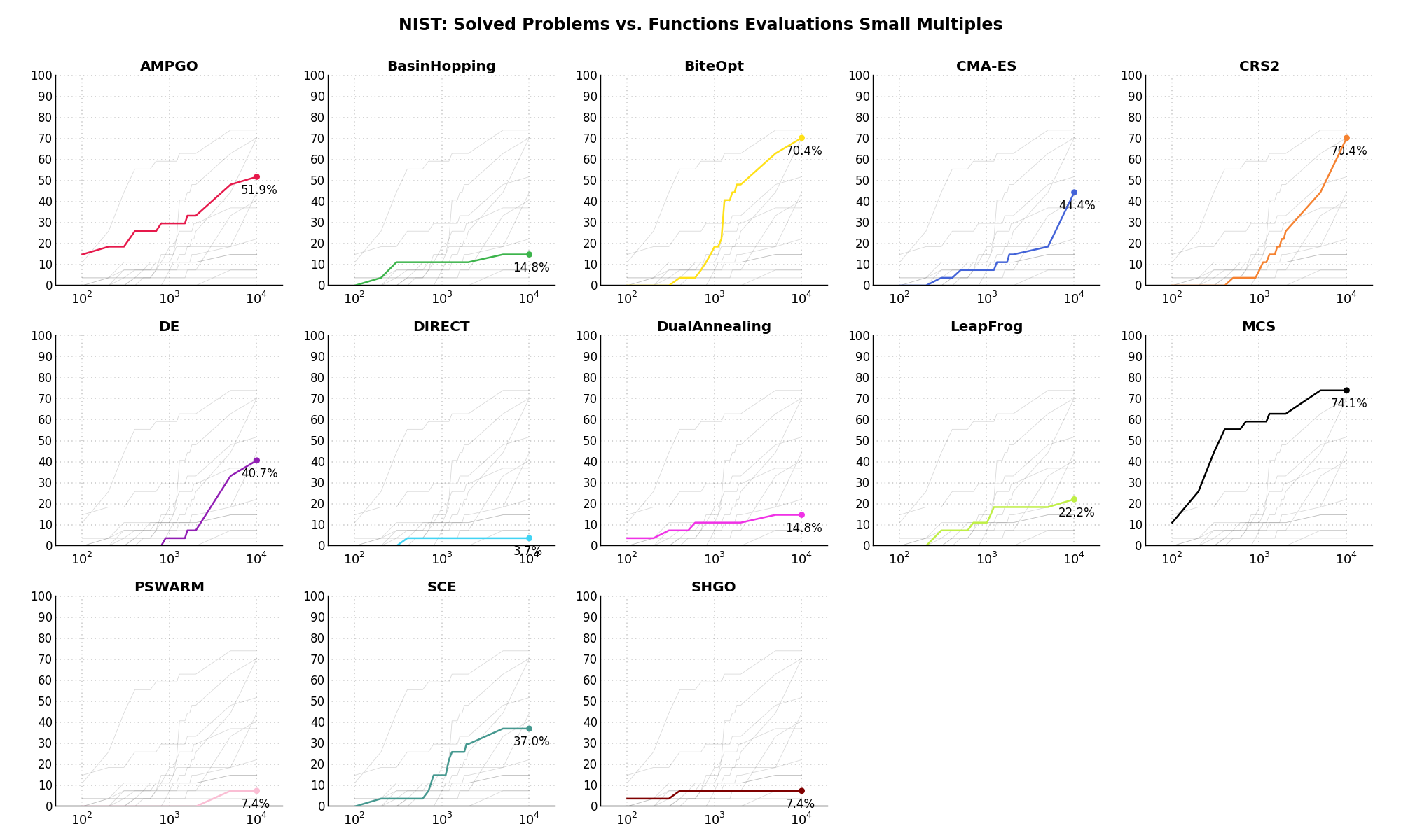
Figure 11.4: Percentage of problems solved given a fixed number of function evaluations on the NIST test suite

The second type of visualization is sometimes referred as “Slopegraph” and there are many variants on the plot layout and appearance that we can implement. The version shown in Figure 11.5 aggregates all the solvers together, so it is easier to spot when a solver overtakes another or the overall performance of an algorithm while the available budget of function evaluations changes.

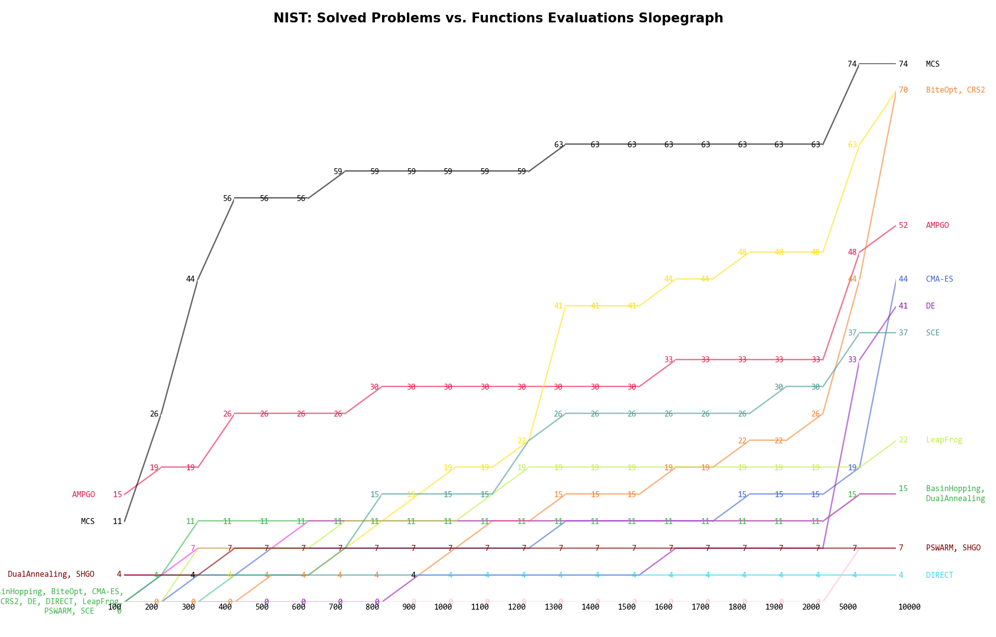
Figure 11.5: Percentage of problems solved given a fixed number of function evaluations on the NIST test suite

A few obvious conclusions we can draw from these pictures are:

For this specific benchmark test suite, no matter your function evaluations budgets, MCS is always going to be the best choice among solvers.
For very large allowances in terms of functions evaluations, then BiteOpt and CRS2 become competitive and they actually share the second place, relatively close to MCS.

NIST¶

Methodology¶

General Solvers Performances¶

Sensitivities on Functions Evaluations Budget¶

Table Of Contents

Previous topic

Next topic

This Page

Navigation

NIST¶

Methodology¶

General Solvers Performances¶

Sensitivities on Functions Evaluations Budget¶

Table Of Contents

Previous topic

Next topic

This Page

Quick search

Navigation