RandomFields¶

F_opt Known	X_opt Known	Difficulty
No	No	Hard

The approach used in the RandomFields test suite is described in https://www.researchgate.net/publication/301940420_Global_optimization_test_problems_based_on_random_field_composition . It generates benchmark functions by “smoothing” one or more multidimensional discrete random fields and composing them, and it is composed by three different steps:

A basic multidimensional discrete random field generator capable to produce parameterized fields with higher order interactions.
A “smoothing” method to obtain continuous and differentiable fields, by means of weighting functions.
A composition technique to create structured fields by combining different types of basic random fields.

No source code is given, but the implementation is fairly straightforward from the article itself.

Methodology¶

For the Multidimensional Discrete Random Field (MDRF) generator, the generator function (referred to as operator $\mathbf{H}$ ), takes a multidimensional vector $\mathbf{x}$ of floating point values from the unit hypercube domain as an input, and maps it to a value from a given set $\mathbf{S}$ with a discrete probability distribution and a computational type (e.g. binary integer or float) of choice:

$y = H(x_1, x_2, x_d, ..., x_n) \: \: \textup{where} \: \: x_d \in [0, 1] \: \: \textup{for} \: \: d=1, 2, ..., n \: \: \textup{and} \: \: y \in \mathbf{S}$

To explain the concept of the implementation, a related discretized version of this idea can be defined as:

$y = A(j_1, j_2, j_d, ..., j_n) \: \: \textup{where} \: \: j_d \in \mathbb{N} \: \: \textup{and} \: \: j_d \leq r_d \: \: \textup{and} \: \: y \in \mathbf{T}$

Operator $\mathbf{A}$ can be interpreted as high-dimensional random “array” A with indices $j$ of which each index $j_d$ is bounded by the maximum array size $r_d$ for dimension $d$ . In the second expression, $\mathbf{T}$ is a finite set of successive integers pointing to the distinct elements of the set $\mathbf{S}$ .

The concept chosen for the MDRF generator algorithm is to compute and reproduce the pseudo-random values of the high-dimensional arrays “on the fly” instead of storing a potentially huge passive map in the computer memory. Another alternative interpretation would be to consider operator :math:A as a pseudorandom number generator with a high-dimensional vector as its generating seed.

Using a multiplicative weighting function as expressed in equation below these discrete random fields can be transformed to “smooth” differentiable continuous random fields:

$\mathbf{C} (\mathbf{x}, \mathbf{r}, \boldsymbol{\varphi}, p) =\left [ \prod_{d=1}^{n} (1 - e^{cos(2\pi(r_d(x_d+\varphi_d)))-1})(\frac{1}{1-e^{-2}}) \right ]^p$

Where $\boldsymbol{\varphi}$ denotes the vector of the (phase) shift of the discrete field and the $\mathbf{C}$ operator such that also fields with non-zero values along the domain boundaries can be constructed ( $\varphi_d \in [0,1]$ ). With parameter $p$ the shape of the function can be adjusted.

The application of the “bare bones” discrete random fields generated by the algorithm above is of little practical interest because of the primitive problem structure. Compositions of such fields of different and heterogeneous resolutions, dimensions and codomain distributions can provide test functions with interesting problem structures. Continuous fields with different spatial resolution can be created, and compositions can be made by for example multiplication or by weighted addition such as for example:

$\mathbf{H_{comp}} (\mathbf{x}) = \sum_{k=1}^{m}w_k \cdot \mathbf{H_{k}} (\mathbf{x}, \mathbf{r_k}, \mathbf{\varphi_k})$

where $\boldsymbol{r_k}$ and $\boldsymbol{\varphi_k}$ (both in bold) denote the vectors with the array size and shifts for each dimension of composition fields $k$ .

To cut the story short, my approach in generating the test functions for the RandomFields benchmarks hs been:

The dimensionality of the problem varies between $N = 2$ and $N = 5$
The number of compositions functions can be 1, 2, 4, 6, 8 or 10
The exponent $p$ can be 0.25, 0.5, 1, 2, or 3
The shift can be any of 0, 0.2, 0.4 or 0.6

In this way, I have generated 120 test functions for each dimension, for a total of 480 benchmarks.

One of the main differences between the RandomFields benchmark and most of the other test suites is that neither the global optimum position nor the actual minimum value of the objective function is known. So, in order to evaluate the solvers performances in a similar way as done previously, I have elected to follow this approach, for each of the 480 functions in the RandomFields test suite:

Generate a brute-force grid of N points between 0 and 1 (the actual bounds). This grid is composed by at least 1,000,000 points (depending on the problem dimensions).
Evaluate the objective function at each of these points.
After identifying the most promising 1,000 points in the grid (i.e., points for which the function value is lowest), start 3 different local optimization algorithms from each of these points. The algorithms selected for this exercise were a mix of derivative-free and gradient-based approaches (L-BFGS-B, Subplex, Power methods).
Out of all these minimizations, the lowest function value obtained becomes the putative “global minimum” for the current benchmark function.

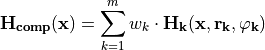
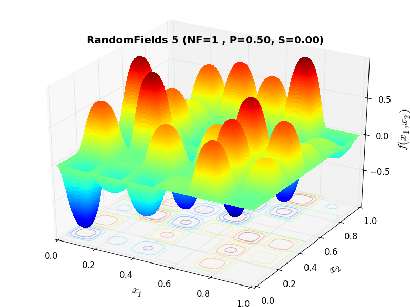
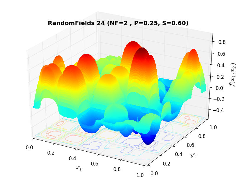
A few examples of 2D benchmark functions created with the RandomFields generator can be seen in Figure 10.1.

RandomFields Function 5	RandomFields Function 24	RandomFields Function 37
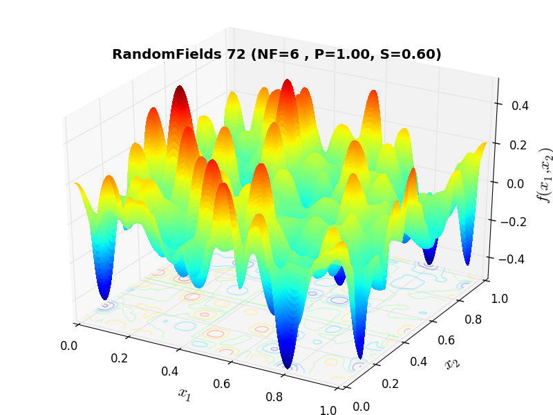
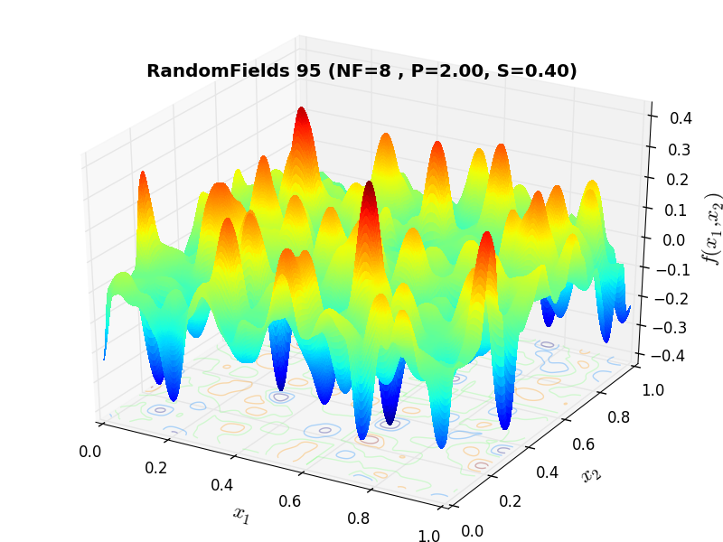
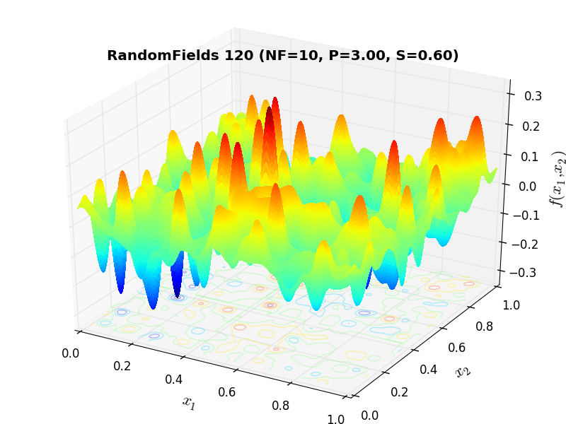
RandomFields Function 72	RandomFields Function 95	RandomFields Function 120

General Solvers Performances¶

Table 10.1 below shows the overall success of all Global Optimization algorithms, considering every benchmark function, for a maximum allowable budget of $NF = 2,000$ .

The RandomFields benchmark suite is a relatively hard test suite: the best solver for $NF = 2,000$ is DIRECT, with a success rate of 34.4%, but DualAnnealing and SHGO achive pretty much the same results, closely followed by MCS.

Note

The reported number of functions evaluations refers to successful optimizations only.

**Table 10.1**: Solvers performances on the RandomFields benchmark suite at NF = 2,000
Optimization Method	Overall Success (%)	Functions Evaluations
AMPGO	10.62%	880
BasinHopping	19.38%	678
BiteOpt	24.79%	598
CMA-ES	9.17%	978
CRS2	13.12%	691
DE	19.79%	1,091
DIRECT	34.38%	435
DualAnnealing	34.17%	510
LeapFrog	8.33%	193
MCS	29.38%	614
PSWARM	14.37%	1,648
SCE	17.08%	786
SHGO	33.96%	513

These results are also depicted in Figure 10.2, which shows that DIRECT, DualAnnealing and SHGO are the better-performing optimization algorithms, followed by MCS.

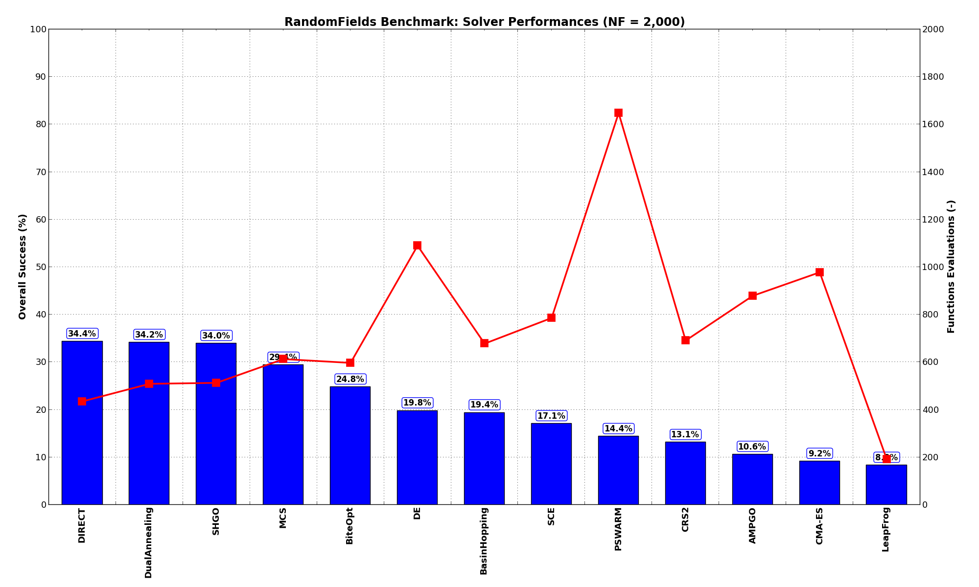
Optimization algorithms performances on the RandomFields test suite at :math:`NF = 2,000`

Figure 10.2: Optimization algorithms performances on the RandomFields test suite at $NF = 2,000$

Pushing the available budget to a very generous 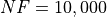$NF = 10,000$ , the results show SHGO taking the lead, with MCS following by a large margin. The results are also shown visually in Figure 10.3.

**Table 10.2**: Solvers performances on the RandomFields benchmark suite at NF = 10,000
Optimization Method	Overall Success (%)	Functions Evaluations
AMPGO	59.17%	2,319
BasinHopping	88.33%	1,312
BiteOpt	38.96%	956
CMA-ES	52.29%	1,665
CRS2	37.08%	1,032
DE	47.08%	1,820
DIRECT	68.75%	962
DualAnnealing	57.29%	791
LeapFrog	23.75%	270
MCS	87.08%	1,614
PSWARM	47.08%	2,110
SCE	43.12%	806
SHGO	80.00%	1,206

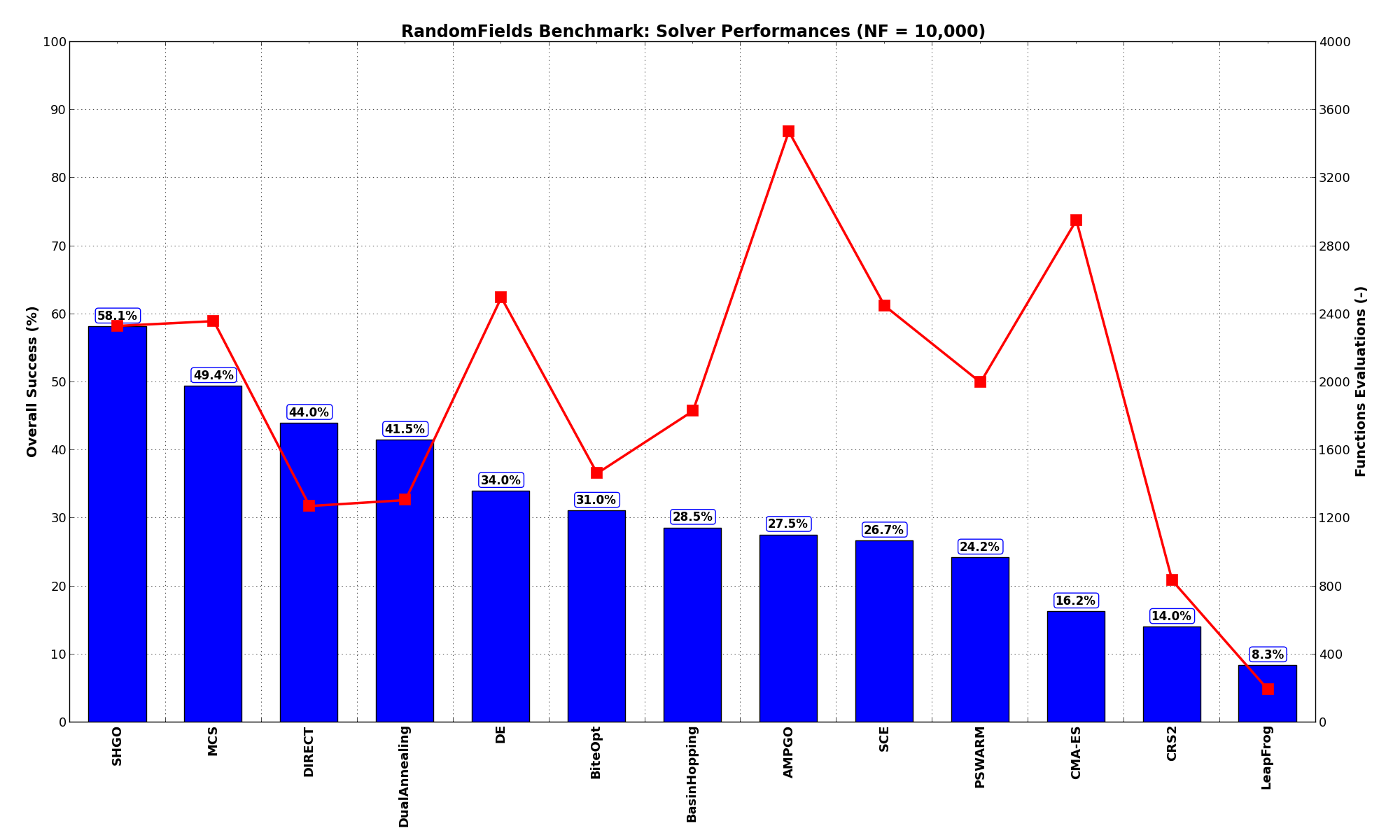
Optimization algorithms performances on the RandomFields test suite at :math:`NF = 10,000`

Figure 10.3: Optimization algorithms performances on the RandomFields test suite at $NF = 10,000$

Sensitivities on Functions Evaluations Budget¶

It is also interesting to analyze the success of an optimization algorithm based on the fraction (or percentage) of problems solved given a fixed number of allowed function evaluations, let’s say 100, 200, 300,... 2000, 5000, 10000.

In order to do that, we can present the results using two different types of visualizations. The first one is some sort of “small multiples” in which each solver gets an individual subplot showing the improvement in the number of solved problems as a function of the available number of function evaluations - on top of a background set of grey, semi-transparent lines showing all the other solvers performances.

This visual gives an indication of how good/bad is a solver compared to all the others as function of the budget available. Results are shown in Figure 10.4.

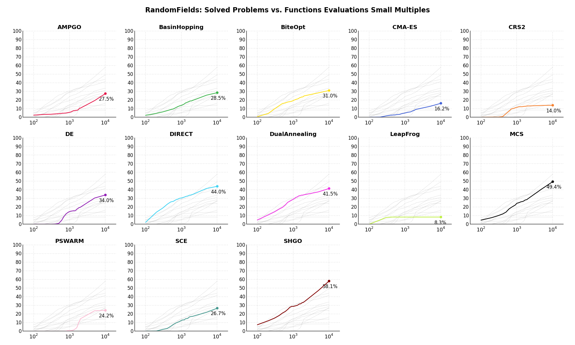
Figure 10.4: Percentage of problems solved given a fixed number of function evaluations on the RandomFields test suite

The second type of visualization is sometimes referred as “Slopegraph” and there are many variants on the plot layout and appearance that we can implement. The version shown in Figure 10.5 aggregates all the solvers together, so it is easier to spot when a solver overtakes another or the overall performance of an algorithm while the available budget of function evaluations changes.

Figure 10.5: Percentage of problems solved given a fixed number of function evaluations on the RandomFields test suite

A few obvious conclusions we can draw from these pictures are:

For this specific benchmark test suite, for lower function evaluations budgets, DIRECT, SHGO and DualAnnealing are the best choices.
The solvers mentioned above keep their lead even at higher function evaluations budgets, although MCS manages to climb back in second place if a large budget is given.

Dimensionality Effects¶

Since I used the RandomFields test suite to generate test functions with dimensionality ranging from 2 to 5, it is interesting to take a look at the solvers performances as a function of the problem dimensionality. Of course, in general it is to be expected that for larger dimensions less problems are going to be solved - although it is not always necessarily so as it also depends on the function being generated. Results are shown in Table 10.3 .

**Table 10.3**: Dimensionality effects on the RandomFields benchmark suite at NF = 2,000
Solver	N = 2	N = 3	N = 4	N = 5	Overall
AMPGO	27.5	8.3	3.3	3.3	10.6
BasinHopping	60.0	11.7	1.7	4.2	19.4
BiteOpt	60.0	20.0	5.8	13.3	24.8
CMA-ES	28.3	6.7	0.8	0.8	9.2
CRS2	40.0	7.5	2.5	2.5	13.1
DE	64.2	15.0	0.0	0.0	19.8
DIRECT	86.7	28.3	12.5	10.0	34.4
DualAnnealing	82.5	29.2	15.8	9.2	34.2
LeapFrog	21.7	6.7	1.7	3.3	8.3
MCS	83.3	17.5	11.7	5.0	29.4
PSWARM	51.7	1.7	0.8	3.3	14.4
SCE	63.3	4.2	0.8	0.0	17.1
SHGO	93.3	23.3	9.2	10.0	34.0

Figure 10.6 shows the same results in a visual way.

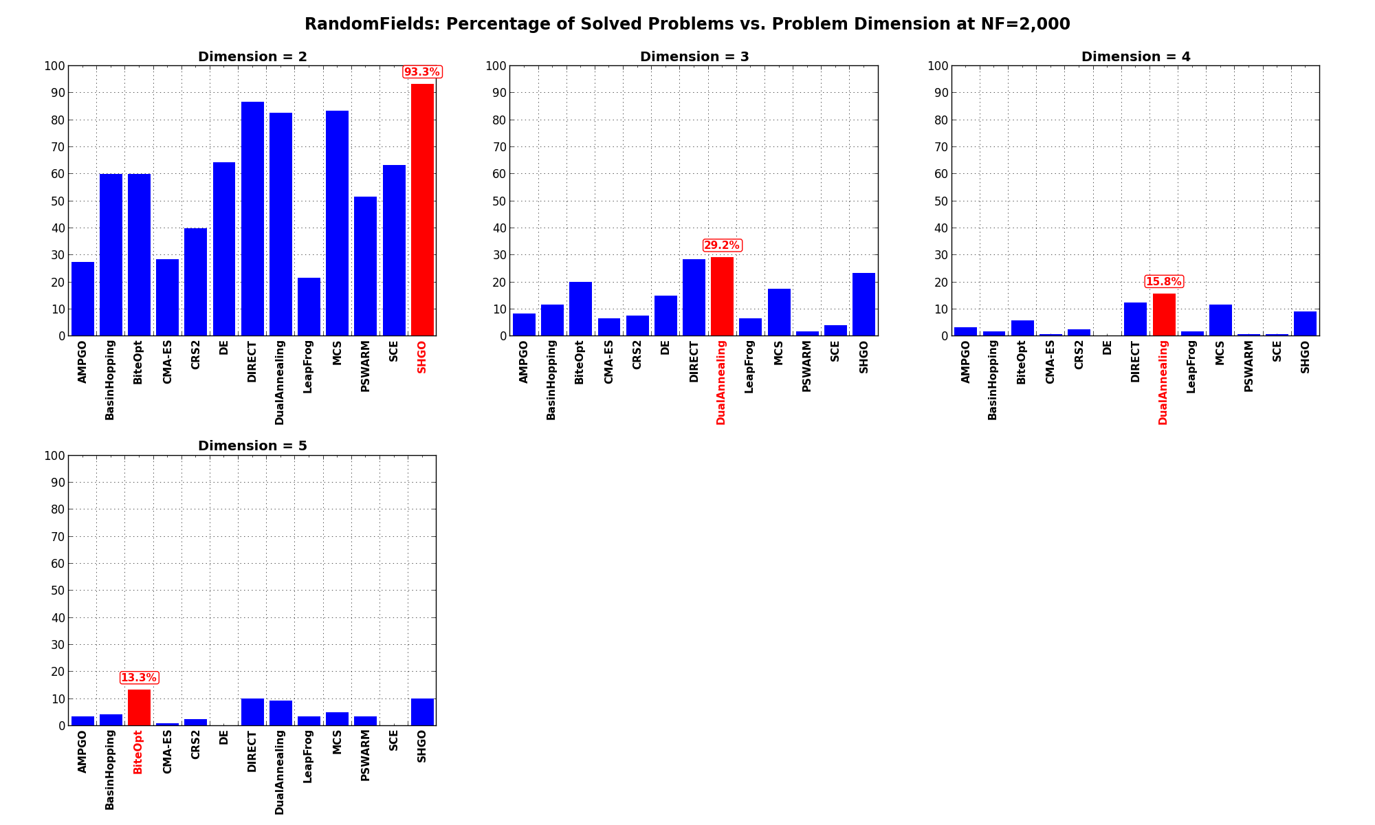
Percentage of problems solved as a function of problem dimension at :math:`NF = 2,000`

Figure 10.6: Percentage of problems solved as a function of problem dimension for the RandomFields test suite at $NF = 2,000$

What we can infer from the table and the figure is that, for low dimensionality problems ( $NF = 2$ ), SHGO is able to solve most of the problems in this test suite, with DIRECT and MCS tightly following. By increasing the dimensionality the performances of all solvers degrade significantly, with DualAnnealing having a marginal advantage over other solvers.

Pushing the available budget to a very generous $NF = 10,000$ shows SHGO solving all problems, with MCS and DIRECT right behind for $N = 2$ . For higher dimensionalities, again performance degradation is evident, although SHGO is the clear winner.

The results for the benchmarks at $NF = 10,000$ are displayed in Table 10.4 and Figure 10.7.

**Table 10.4**: Dimensionality effects on the RandomFields benchmark suite at NF = 10,000
Solver	N = 2	N = 3	N = 4	N = 5	Overall
AMPGO	72.5	21.7	5.0	10.8	27.5
BasinHopping	73.3	24.2	6.7	10.0	28.5
BiteOpt	75.0	24.2	8.3	16.7	31.0
CMA-ES	43.3	11.7	5.8	4.2	16.2
CRS2	40.0	8.3	4.2	3.3	14.0
DE	64.2	40.0	25.8	5.8	34.0
DIRECT	95.8	42.5	17.5	20.0	44.0
DualAnnealing	85.8	39.2	24.2	16.7	41.5
LeapFrog	21.7	6.7	1.7	3.3	8.3
MCS	98.3	58.3	25.0	15.8	49.4
PSWARM	66.7	17.5	6.7	5.8	24.2
SCE	76.7	22.5	6.7	0.8	26.7
SHGO	100.0	66.7	23.3	42.5	58.1

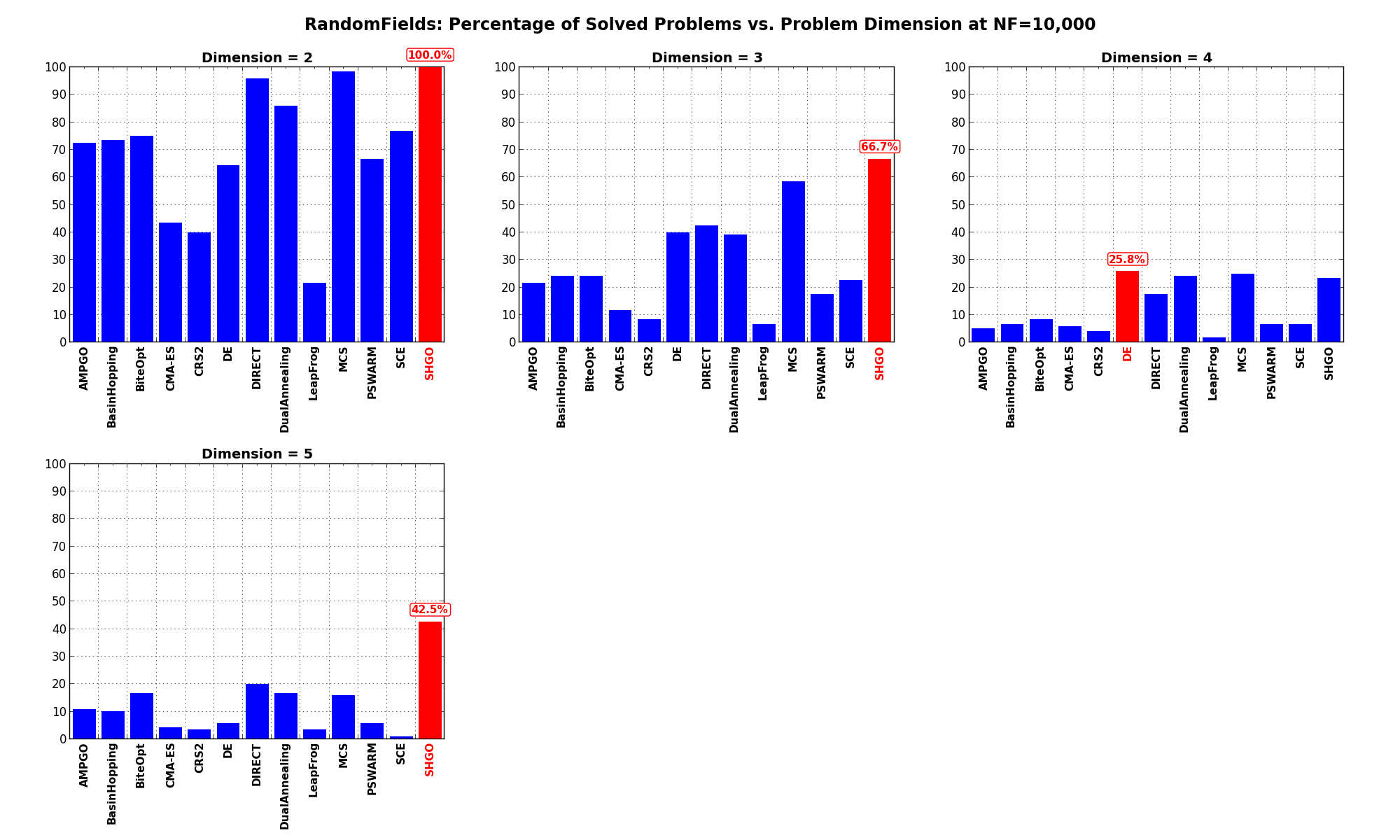
Percentage of problems solved as a function of problem dimension at :math:`NF = 10,000`

Figure 10.7: Percentage of problems solved as a function of problem dimension for the RandomFields test suite at $NF = 10,000$

RandomFields¶

Methodology¶

General Solvers Performances¶

Sensitivities on Functions Evaluations Budget¶

Dimensionality Effects¶

Table Of Contents

Previous topic

Next topic

This Page

Navigation

RandomFields¶

Methodology¶

General Solvers Performances¶

Sensitivities on Functions Evaluations Budget¶

Dimensionality Effects¶

Table Of Contents

Previous topic

Next topic

This Page

Quick search

Navigation