MPM2¶

F_opt Known	X_opt Known	Difficulty
Yes	Yes	Medium

Many test problems in real-valued optimization do not provide information about important problem properties, as, e. g., the positions of all local optima and the corresponding attraction basins. Knowing these characteristics would be helpful in many cases of benchmarking of optimization algorithms. Since many authors suggested to use parametrized problem generators that can produce test instances randomly but with controllable difficulty, several problem formulations appeared for which these new requirements can be handled well. The common ground of all these is that the objective function is generated by taking the maximum or minimum of several unimodal functions.

The implementation of this test function generator is described in detail in https://ls11-www.cs.tu-dortmund.de/_media/techreports/tr15-01.pdf .

Methodology¶

The “Multiple Peaks Model 2” (MPM2) test suite produces multimodal problem instances by combining several randomly distributed peaks. Hence, the problems are irregular and non-separable, which are also important features of difficult real-world problems. The problem is defined by the following formulas:

$f(\mathbf{x}) = 1 - \max \left \{ g(\mathbf{x}, \mathbf{p}) \mid \mathbf{p} \in P \right \} \\ \\ g(\mathbf{x}, \mathbf{p}) = \frac{h_p}{1+\frac{md(\mathbf{x}, \mathbf{p})^{s_p}}{r_p}} \\ \\ md(\mathbf{x}, \mathbf{p}) = \sqrt{(\mathbf{x} - \mathbf{p})^T \Sigma_{p}^{-1}(\mathbf{x} - \mathbf{p})} \\$

The objective function is given in the first equation. It takes the minimum of $N_{peaks} = \mid P \mid$ unimodal functions (from the second equation) around peak positions $\mathbf{p} \in P$ . This has the advantage that local optima with known positions are created, which is necessary to calculate some quality indicators.

Each of these functions is associated with parameters $h_p$ , $s_p$ , and $r_p$ for height, shape, and radius, respectively. By slightly deviating from locally quadratic behavior ( $s_p = 2$ ), the test suite intends to increase the difficulty for local search algorithms. Radii $r_p$ influence the size of attraction basins, and thus the probability to place a starting point in the basin. Optima with small attraction basins will be difficult to find. Additionally, a randomly drawn covariance matrix $\Sigma_p$ belongs to each peak. This matrix is used to create the optima’s basins as rotated hyperellipsoids, by calculating the Mahalanobis distance in the third equation.

That said, my approach to generate test functions for this benchmark has been the following:

The dimensionality of the problem varies between $N = 2$ and $N = 5$
The number of peaks can be any of 5, 10, 20, 50 or 100
The topology of the peaks can be defined either as “funnel” or as “random”
The shape size an height can be correlated, anti-correlated or uncorrelated
Shapes can be rotated or not
Finally, the shape used can be ellipses or spheres.

With all these variable settings, I generated 120 valid test function per dimension, thus the current MPM2 test suite contains 480 benchmark functions.

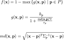
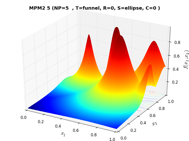
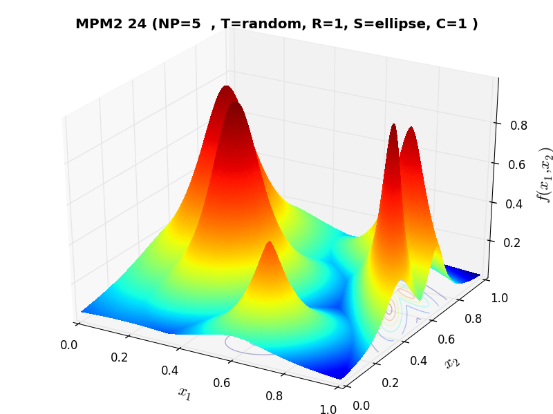
A few examples of 2D benchmark functions created with the MPM2 generator can be seen in Figure 9.1.

MPM2 Function 5	MPM2 Function 24	MPM2 Function 37
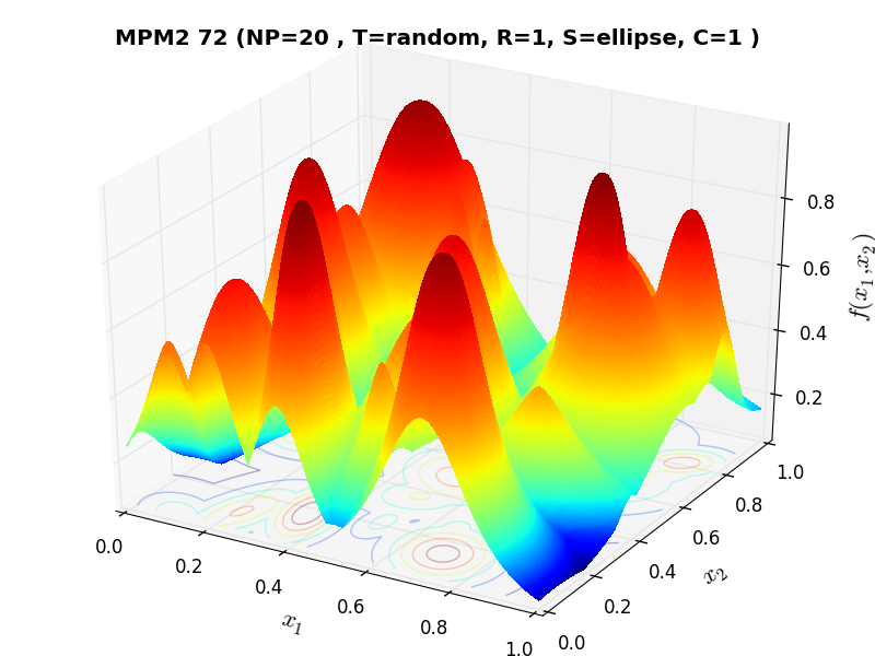
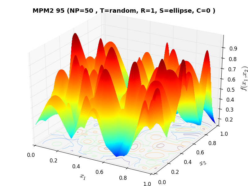
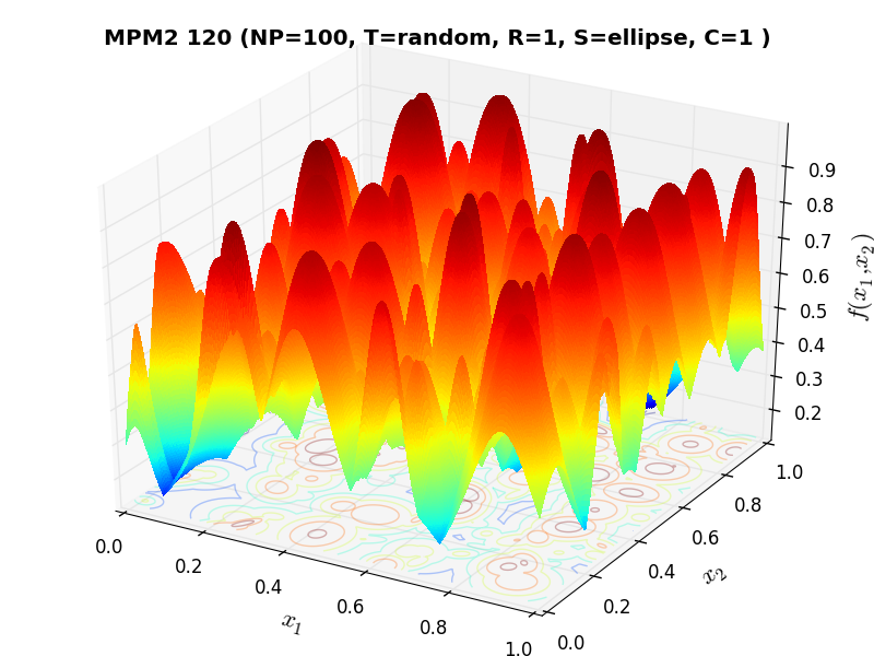
MPM2 Function 72	MPM2 Function 95	MPM2 Function 120

General Solvers Performances¶

Table 9.1 below shows the overall success of all Global Optimization algorithms, considering every benchmark function, for a maximum allowable budget of $NF = 2,000$ .

The MPM2 benchmark suite is a relatively easy test suite: the best solver for $NF = 2,000$ is BasinHopping, with a success rate of 68.1%, closely followed by MCS and SHGO.

Note

The reported number of functions evaluations refers to successful optimizations only.

**Table 9.1**: Solvers performances on the MPM2 benchmark suite at NF = 2,000
Optimization Method	Overall Success (%)	Functions Evaluations
AMPGO	36.04%	660
BasinHopping	68.12%	522
BiteOpt	35.00%	462
CMA-ES	39.58%	750
CRS2	35.00%	946
DE	32.92%	1,170
DIRECT	59.79%	464
DualAnnealing	50.62%	376
LeapFrog	23.75%	270
MCS	65.62%	580
PSWARM	21.25%	1,595
SCE	40.83%	588
SHGO	65.21%	510

These results are also depicted in Figure 9.2, which shows that BasinHopping is the better-performing optimization algorithm, followed by MCS and SHGO.

Optimization algorithms performances on the MPM2 test suite at :math:`NF = 2,000`

Figure 9.2: Optimization algorithms performances on the MPM2 test suite at $NF = 2,000$

Pushing the available budget to a very generous $NF = 10,000$ , the results show BasinHopping still keeping the lead, with MCS much closer now and SHGO trailing a bit behind. The results are also shown visually in Figure 9.3.

**Table 9.2**: Solvers performances on the MPM2 benchmark suite at NF = 10,000
Optimization Method	Overall Success (%)	Functions Evaluations
AMPGO	59.17%	2,319
BasinHopping	88.33%	1,312
BiteOpt	38.96%	956
CMA-ES	52.29%	1,665
CRS2	37.08%	1,032
DE	47.08%	1,820
DIRECT	68.75%	962
DualAnnealing	57.29%	791
LeapFrog	23.75%	270
MCS	87.08%	1,614
PSWARM	47.08%	2,110
SCE	43.12%	806
SHGO	80.00%	1,206

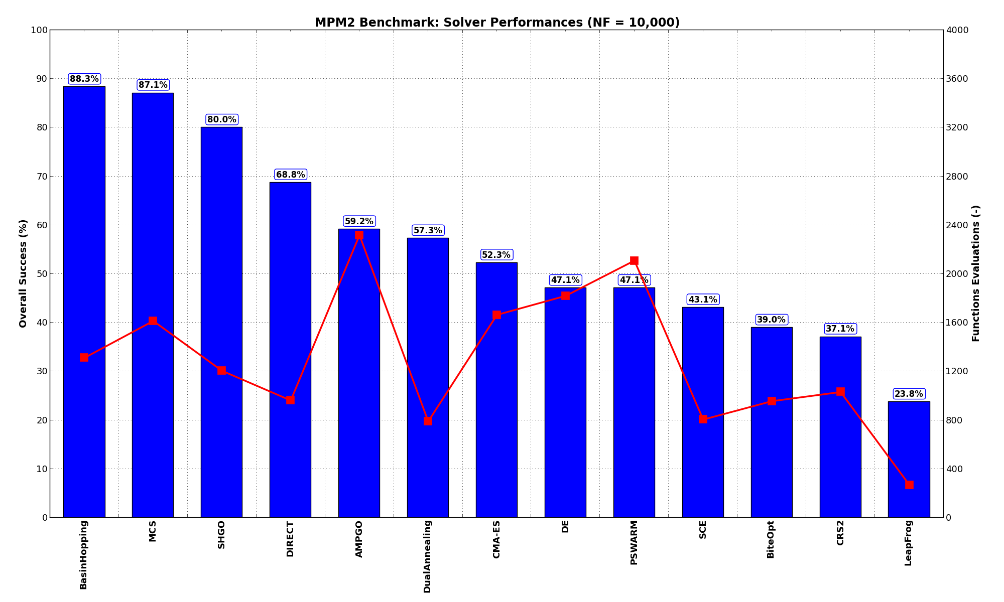
Optimization algorithms performances on the MPM2 test suite at :math:`NF = 10,000`

Figure 9.3: Optimization algorithms performances on the MPM2 test suite at $NF = 10,000$

Sensitivities on Functions Evaluations Budget¶

It is also interesting to analyze the success of an optimization algorithm based on the fraction (or percentage) of problems solved given a fixed number of allowed function evaluations, let’s say 100, 200, 300,... 2000, 5000, 10000.

In order to do that, we can present the results using two different types of visualizations. The first one is some sort of “small multiples” in which each solver gets an individual subplot showing the improvement in the number of solved problems as a function of the available number of function evaluations - on top of a background set of grey, semi-transparent lines showing all the other solvers performances.

This visual gives an indication of how good/bad is a solver compared to all the others as function of the budget available. Results are shown in Figure 9.4.

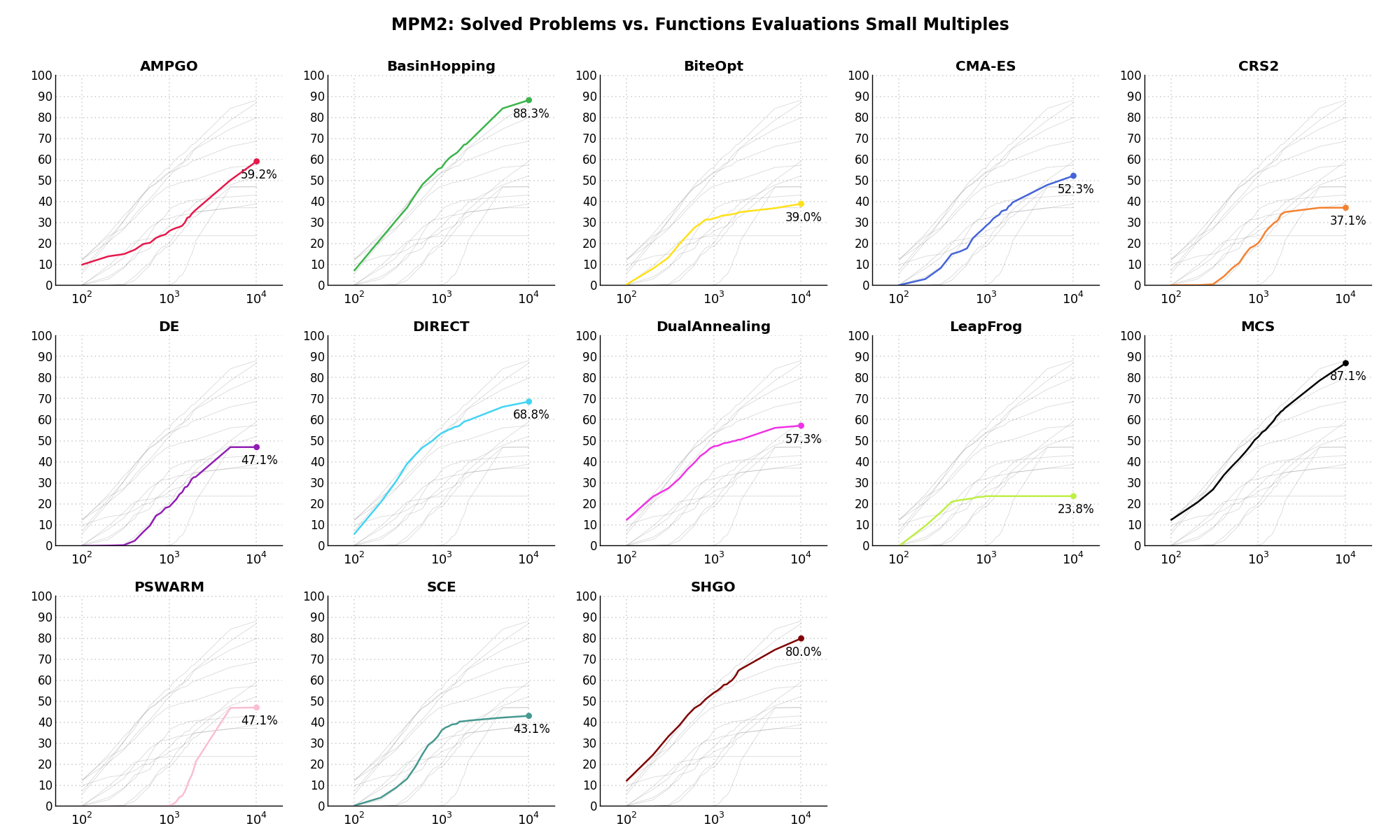
Figure 9.4: Percentage of problems solved given a fixed number of function evaluations on the MPM2 test suite

The second type of visualization is sometimes referred as “Slopegraph” and there are many variants on the plot layout and appearance that we can implement. The version shown in Figure 9.5 aggregates all the solvers together, so it is easier to spot when a solver overtakes another or the overall performance of an algorithm while the available budget of function evaluations changes.

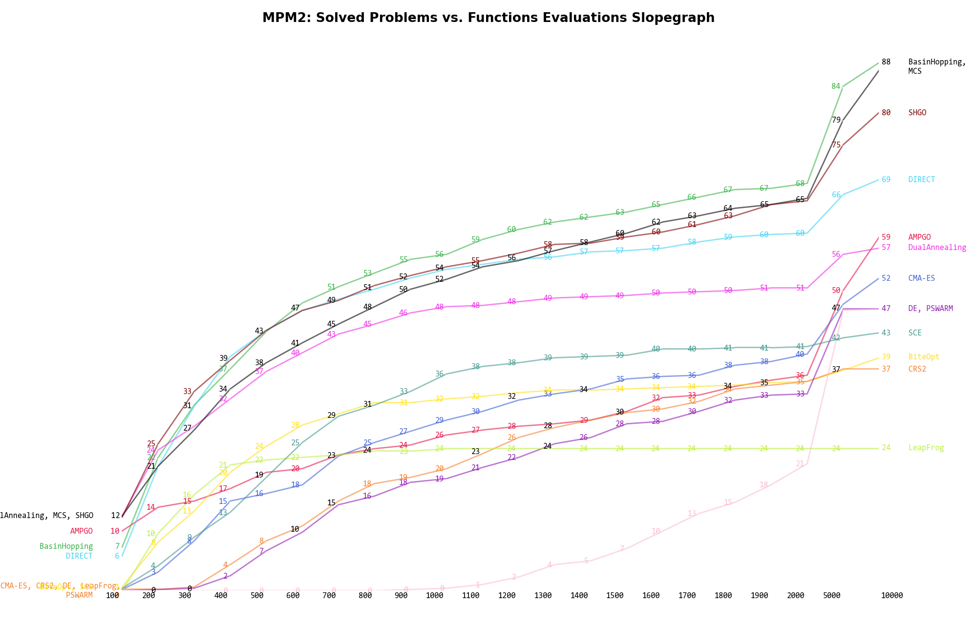
Figure 9.5: Percentage of problems solved given a fixed number of function evaluations on the MPM2 test suite

A few obvious conclusions we can draw from these pictures are:

For this specific benchmark test suite, for very limited function evaluations budgets, BasinHopping, SHGO and DIRECT are the best choices, tightly followed by MCS.
The solvers mentioned above keep their lead even at higher function evaluations budgets, although BasinHopping manages to stay on top at every step.

Dimensionality Effects¶

Since I used the MPM2 test suite to generate test functions with dimensionality ranging from 2 to 5, it is interesting to take a look at the solvers performances as a function of the problem dimensionality. Of course, in general it is to be expected that for larger dimensions less problems are going to be solved - although it is not always necessarily so as it also depends on the function being generated. Results are shown in Table 9.3 .

**Table 9.3**: Dimensionality effects on the MPM2 benchmark suite at NF = 2,000
Solver	N = 2	N = 3	N = 4	N = 5	Overall
AMPGO	65.8	32.5	29.2	16.7	36.0
BasinHopping	94.2	70.0	62.5	45.8	68.1
BiteOpt	68.3	28.3	27.5	15.8	35.0
CMA-ES	63.3	41.7	35.8	17.5	39.6
CRS2	59.2	37.5	31.7	11.7	35.0
DE	74.2	49.2	8.3	0.0	32.9
DIRECT	96.7	75.0	49.2	18.3	59.8
DualAnnealing	83.3	52.5	40.8	25.8	50.6
LeapFrog	46.7	14.2	16.7	17.5	23.8
MCS	95.0	75.8	53.3	38.3	65.6
PSWARM	55.0	20.0	8.3	1.7	21.2
SCE	71.7	40.8	30.8	20.0	40.8
SHGO	95.8	61.7	62.5	40.8	65.2

Figure 9.6 shows the same results in a visual way.

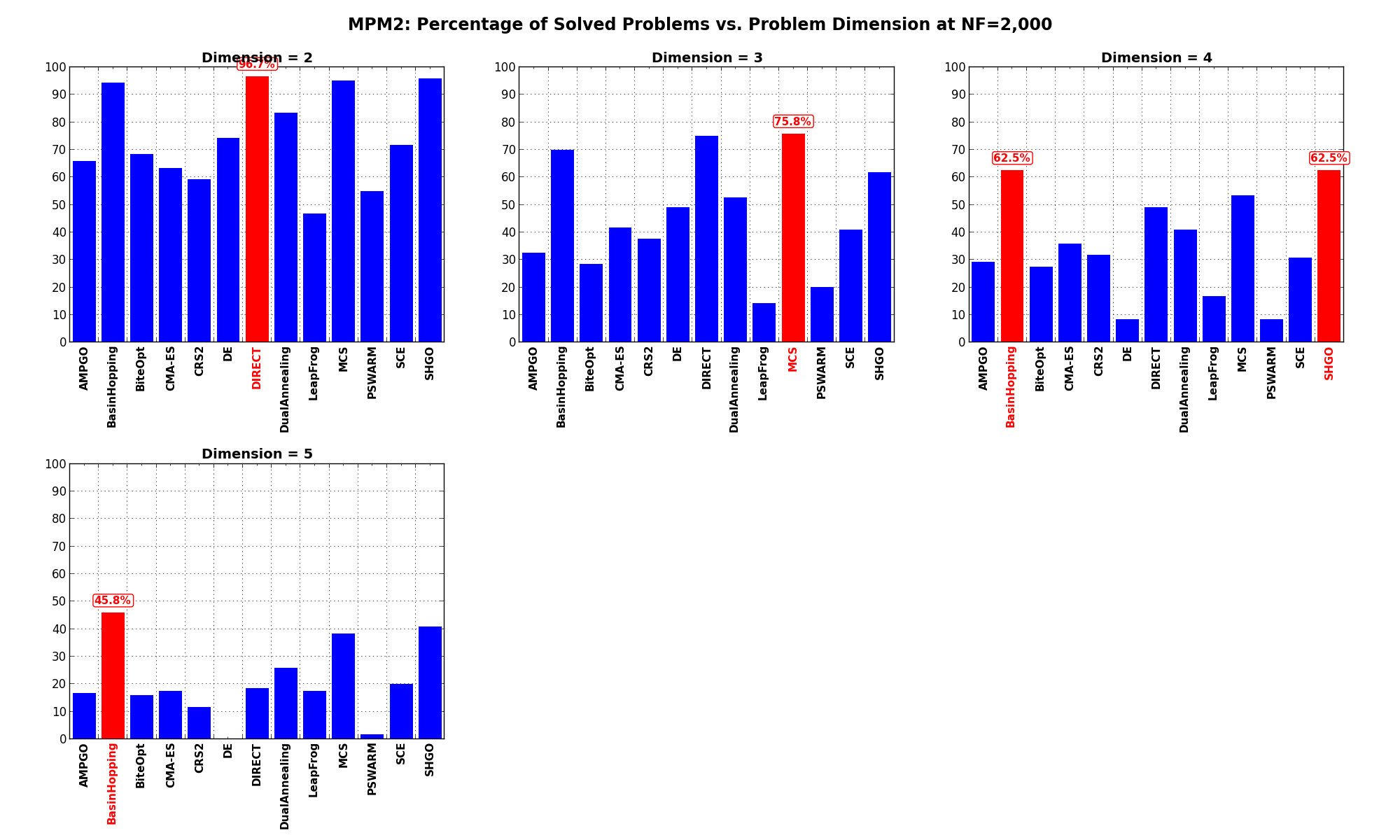
Percentage of problems solved as a function of problem dimension at :math:`NF = 2,000`

Figure 9.6: Percentage of problems solved as a function of problem dimension for the MPM2 test suite at $NF = 2,000$

What we can infer from the table and the figure is that, for low dimensionality problems ( $NF = 2$ ), very many solvers are able to solve most of the problems in this test suite, with DIRECT leading the pack. By increasing the dimensionality other solvers catch up ( MCS, SHGO and BasinHopping).

Pushing the available budget to a very generous $NF = 10,000$ shows MCS and DIRECT solving all problems for $N = 2$ . MCS remains competitive even at higher dimensions but BasinHopping is the clear winner on all problems.

The results for the benchmarks at $NF = 10,000$ are displayed in Table 9.4 and Figure 9.7.

**Table 9.4**: Dimensionality effects on the MPM2 benchmark suite at NF = 10,000
Solver	N = 2	N = 3	N = 4	N = 5	Overall
AMPGO	86.7	60.8	50.0	39.2	59.2
BasinHopping	96.7	93.3	86.7	76.7	88.3
BiteOpt	74.2	36.7	29.2	15.8	39.0
CMA-ES	70.0	51.7	49.2	38.3	52.3
CRS2	59.2	38.3	31.7	19.2	37.1
DE	74.2	54.2	39.2	20.8	47.1
DIRECT	100.0	78.3	64.2	32.5	68.8
DualAnnealing	91.7	64.2	43.3	30.0	57.3
LeapFrog	46.7	14.2	16.7	17.5	23.8
MCS	100.0	93.3	80.8	74.2	87.1
PSWARM	78.3	49.2	37.5	23.3	47.1
SCE	73.3	46.7	32.5	20.0	43.1
SHGO	99.2	83.3	68.3	69.2	80.0

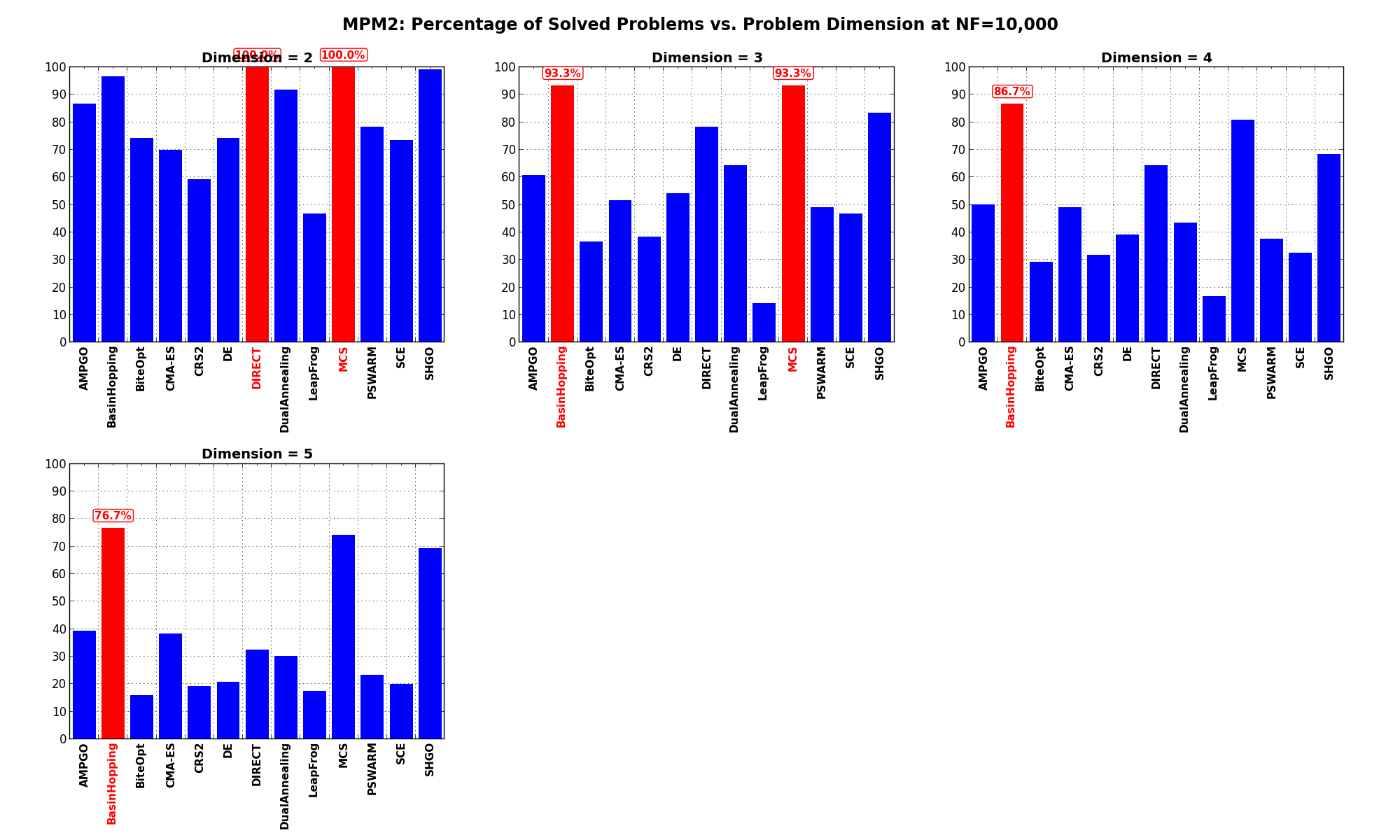
Percentage of problems solved as a function of problem dimension at :math:`NF = 10,000`

Figure 9.7: Percentage of problems solved as a function of problem dimension for the MPM2 test suite at $NF = 10,000$

MPM2¶

Methodology¶

General Solvers Performances¶

Sensitivities on Functions Evaluations Budget¶

Dimensionality Effects¶

Table Of Contents

Previous topic

Next topic

This Page

Navigation

MPM2¶

Methodology¶

General Solvers Performances¶

Sensitivities on Functions Evaluations Budget¶

Dimensionality Effects¶

Table Of Contents

Previous topic

Next topic

This Page

Quick search

Navigation