NgLi¶

F_opt Known	X_opt Known	Difficulty
Yes	Yes	Easy

Stemming from the work of Chi-Kong Ng and Duan Li, this is a test problem generator for unconstrained optimization, but it’s fairly easy to assign bound constraints to it. The methodology is described in https://www.sciencedirect.com/science/article/pii/S0305054814001774 , while the Matlab source code can be found in http://www1.se.cuhk.edu.hk/~ckng/generator/ .

Methodology¶

I don’t think I will be able to summarize the maths behind this test function generator, so I refer the reader to the paper linked in the introduction. I have used the Matlab script to generate 240 problems with dimensionality varying from 2 to 5 by outputting the generator parameters in text files, then used Python to create the objective functions based on those parameters and the benchmark methodology.

A few examples of 2D benchmark functions created with the NgLi generator can be seen in Figure 8.1.

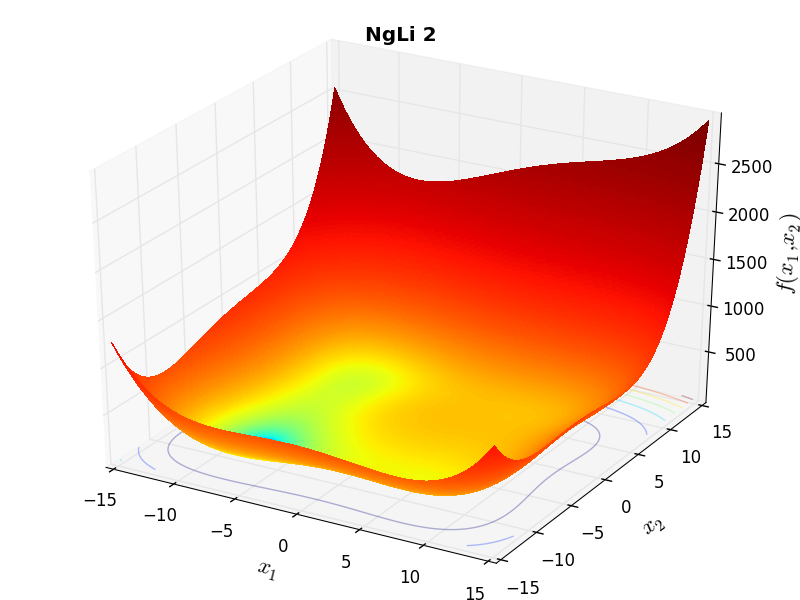
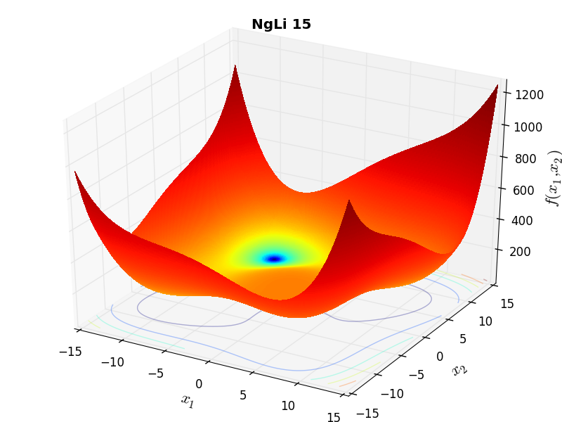
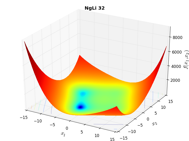
NgLi Function 2	NgLi Function 15	NgLi Function 32
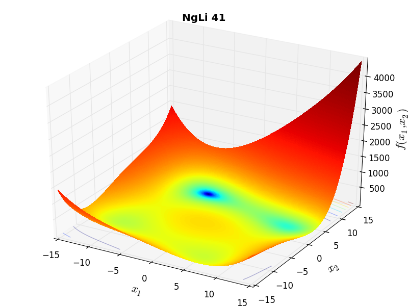
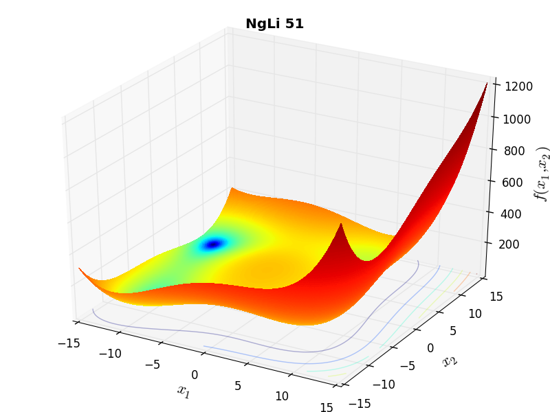
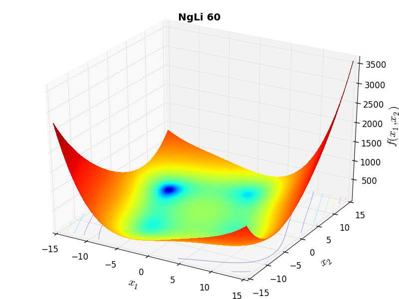
NgLi Function 41	NgLi Function 51	NgLi Function 60

General Solvers Performances¶

Table 8.1 below shows the overall success of all Global Optimization algorithms, considering every benchmark function, for a maximum allowable budget of $NF = 2,000$ .

The NgLi benchmark suite is a relatively easy test suite: the best solver for $NF = 2,000$ is MCS, with a success rate of 86.7%, closely followed by SCE and SHGO.

Note

The reported number of functions evaluations refers to successful optimizations only.

**Table 8.1**: Solvers performances on the NgLi benchmark suite at NF = 2,000
Optimization Method	Overall Success (%)	Functions Evaluations
AMPGO	59.58%	579
BasinHopping	32.50%	176
BiteOpt	51.67%	473
CMA-ES	56.25%	762
CRS2	61.67%	1,206
DE	43.33%	1,282
DIRECT	59.58%	636
DualAnnealing	68.75%	242
LeapFrog	42.92%	304
MCS	86.67%	343
PSWARM	2.50%	1,834
SCE	77.92%	571
SHGO	75.83%	304

These results are also depicted in Figure 8.2, which shows that MCS is the better-performing optimization algorithm, followed by SCE and SHGO.

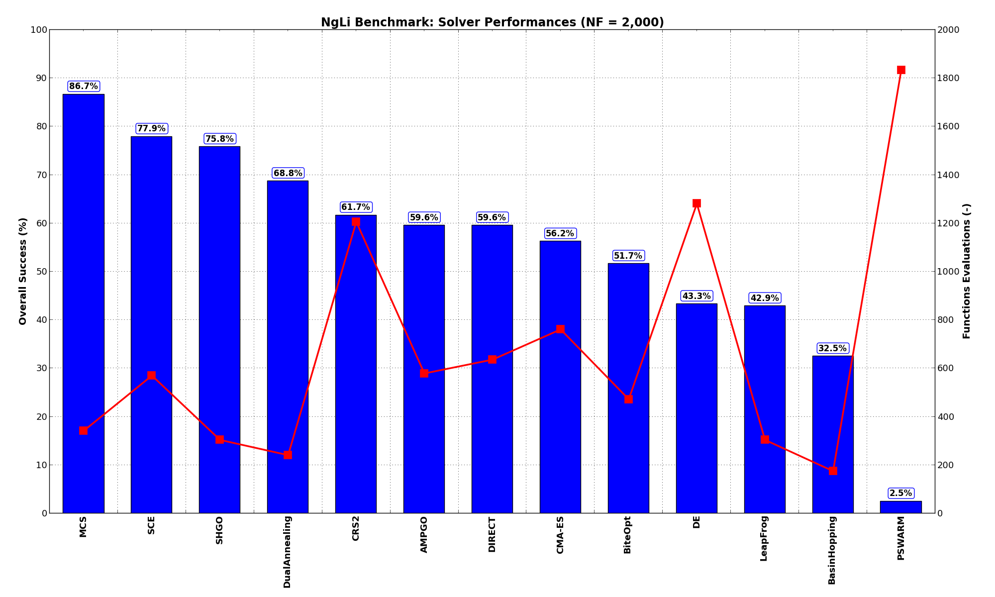
Optimization algorithms performances on the NgLi test suite at :math:`NF = 2,000`

Figure 8.2: Optimization algorithms performances on the NgLi test suite at $NF = 2,000$

Pushing the available budget to a very generous $NF = 10,000$ , the results show MCS basically solving the vast majority of problems (more than 96%), followed at a distance by SHGO and DE. The results are also shown visually in Figure 8.3.

**Table 8.2**: Solvers performances on the NgLi benchmark suite at NF = 10,000
Optimization Method	Overall Success (%)	Functions Evaluations
AMPGO	85.42%	1,939
BasinHopping	33.33%	254
BiteOpt	54.58%	682
CMA-ES	82.08%	1,804
CRS2	79.17%	1,527
DE	82.50%	2,623
DIRECT	76.25%	1,463
DualAnnealing	72.92%	437
LeapFrog	42.92%	304
MCS	96.25%	730
PSWARM	75.42%	2,786
SCE	79.58%	700
SHGO	84.58%	758

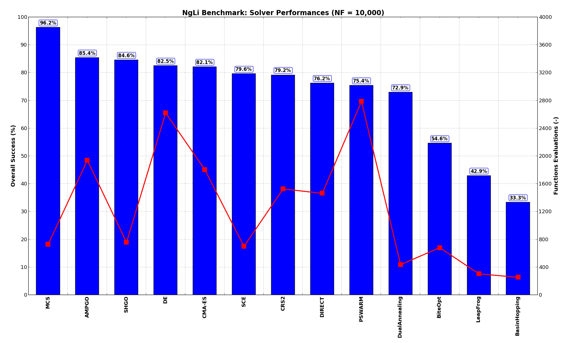
Optimization algorithms performances on the NgLi test suite at :math:`NF = 10,000`

Figure 8.3: Optimization algorithms performances on the NgLi test suite at $NF = 10,000$

Sensitivities on Functions Evaluations Budget¶

It is also interesting to analyze the success of an optimization algorithm based on the fraction (or percentage) of problems solved given a fixed number of allowed function evaluations, let’s say 100, 200, 300,... 2000, 5000, 10000.

In order to do that, we can present the results using two different types of visualizations. The first one is some sort of “small multiples” in which each solver gets an individual subplot showing the improvement in the number of solved problems as a function of the available number of function evaluations - on top of a background set of grey, semi-transparent lines showing all the other solvers performances.

This visual gives an indication of how good/bad is a solver compared to all the others as function of the budget available. Results are shown in Figure 8.4.

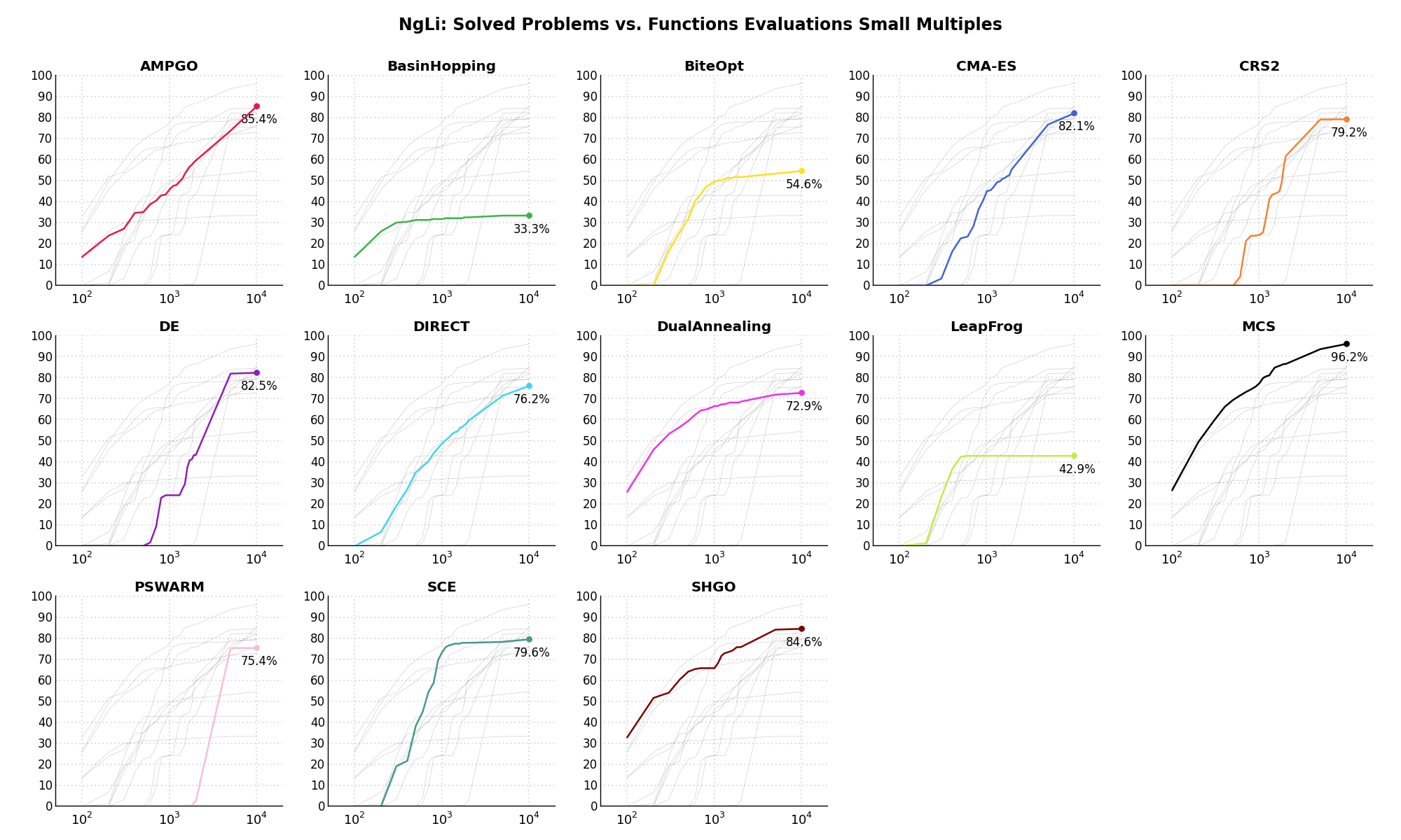
Figure 8.4: Percentage of problems solved given a fixed number of function evaluations on the NgLi test suite

The second type of visualization is sometimes referred as “Slopegraph” and there are many variants on the plot layout and appearance that we can implement. The version shown in Figure 8.5 aggregates all the solvers together, so it is easier to spot when a solver overtakes another or the overall performance of an algorithm while the available budget of function evaluations changes.

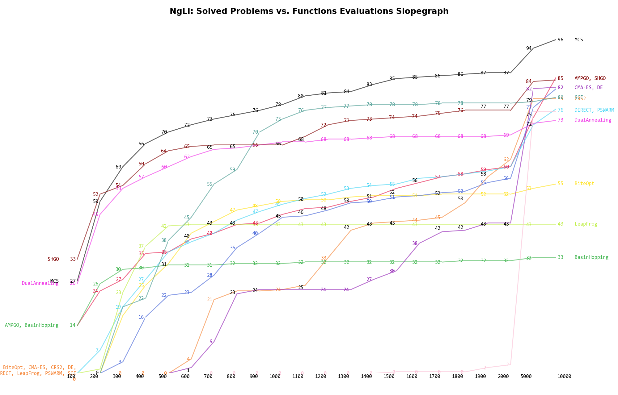
Figure 8.5: Percentage of problems solved given a fixed number of function evaluations on the NgLi test suite

A few obvious conclusions we can draw from these pictures are:

For this specific benchmark test suite, irrespective of your function evaluations budget, MCS will always deliver best performances, but one can do well in choosing also SHGO or DualAnnealing.
While quite a few algorithms benefit from increasing the budget of available function evaluations (CMA-ES, DE), the improvement of PSWARM is unbelievable - from 2% To 76% of problems solved.

Dimensionality Effects¶

Since I used the NgLi test suite to generate test functions with dimensionality ranging from 2 to 5, it is interesting to take a look at the solvers performances as a function of the problem dimensionality. Of course, in general it is to be expected that for larger dimensions less problems are going to be solved - although it is not always necessarily so as it also depends on the function being generated. Results are shown in Table 8.3 .

**Table 8.3**: Dimensionality effects on the NgLi benchmark suite at NF = 2,000
Solver	N = 2	N = 3	N = 4	N = 5	Overall
AMPGO	100.0	71.7	50.0	16.7	59.6
BasinHopping	50.0	31.7	23.3	25.0	32.5
BiteOpt	88.3	53.3	45.0	20.0	51.7
CMA-ES	80.0	66.7	46.7	31.7	56.2
CRS2	95.0	80.0	71.7	0.0	61.7
DE	96.7	76.7	0.0	0.0	43.3
DIRECT	100.0	96.7	36.7	5.0	59.6
DualAnnealing	100.0	85.0	51.7	38.3	68.8
LeapFrog	78.3	36.7	38.3	18.3	42.9
MCS	100.0	100.0	83.3	63.3	86.7
PSWARM	10.0	0.0	0.0	0.0	2.5
SCE	91.7	85.0	71.7	63.3	77.9
SHGO	100.0	100.0	75.0	28.3	75.8

Figure 8.6 shows the same results in a visual way.

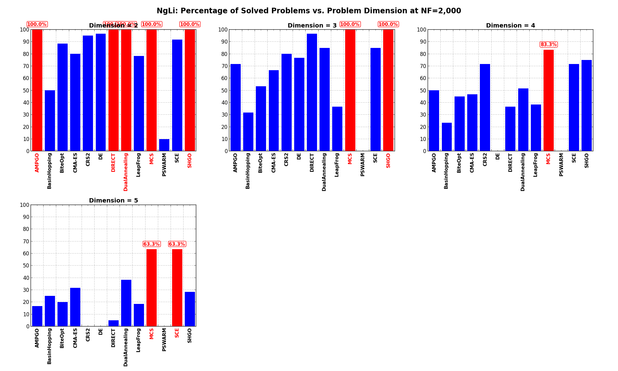
Percentage of problems solved as a function of problem dimension at :math:`NF = 2,000`

Figure 8.6: Percentage of problems solved as a function of problem dimension for the NgLi test suite at $NF = 2,000$

What we can infer from the table and the figure is that, for low dimensionality problems ( $NF = 2$ ), very many solvers are able to solve all problems in this test suite. Increasing the dimensionality makes MCS stand out compared to other solvers.

Pushing the available budget to a very generous $NF = 10,000$ shows a similar trend, with the obvious improvements from CMA-ES and PSWARM.

The results for the benchmarks at $NF = 10,000$ are displayed in Table 8.4 and Figure 8.7.

**Table 8.4**: Dimensionality effects on the NgLi benchmark suite at NF = 10,000
Solver	N = 2	N = 3	N = 4	N = 5	Overall
AMPGO	100.0	96.7	88.3	56.7	85.4
BasinHopping	50.0	33.3	23.3	26.7	33.3
BiteOpt	91.7	60.0	45.0	21.7	54.6
CMA-ES	85.0	76.7	80.0	86.7	82.1
CRS2	95.0	80.0	78.3	63.3	79.2
DE	96.7	78.3	81.7	73.3	82.5
DIRECT	100.0	100.0	78.3	26.7	76.2
DualAnnealing	100.0	88.3	58.3	45.0	72.9
LeapFrog	78.3	36.7	38.3	18.3	42.9
MCS	100.0	100.0	98.3	86.7	96.2
PSWARM	98.3	81.7	68.3	53.3	75.4
SCE	98.3	85.0	71.7	63.3	79.6
SHGO	100.0	100.0	75.0	63.3	84.6

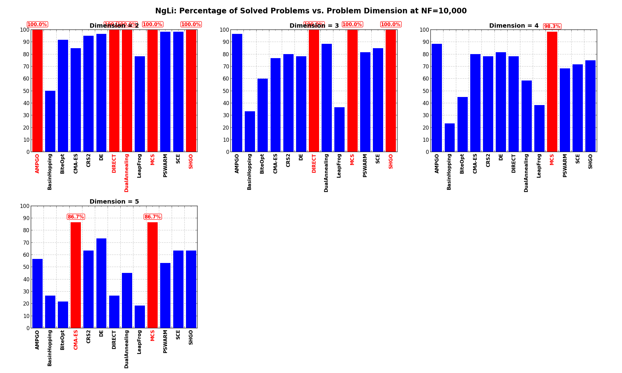
Percentage of problems solved as a function of problem dimension at :math:`NF = 10,000`

Figure 8.7: Percentage of problems solved as a function of problem dimension for the NgLi test suite at $NF = 10,000$

NgLi¶

Methodology¶

General Solvers Performances¶

Sensitivities on Functions Evaluations Budget¶

Dimensionality Effects¶

Table Of Contents

Previous topic

Next topic

This Page

Navigation

NgLi¶

Methodology¶

General Solvers Performances¶

Sensitivities on Functions Evaluations Budget¶

Dimensionality Effects¶

Table Of Contents

Previous topic

Next topic

This Page

Quick search

Navigation