GOTPY¶

F_opt Known	X_opt Known	Difficulty
Yes	Yes	Hard

The GOTPY is another test function generator, pretty much unknown and unused by anyone I could find on the web. There is relatively scant information on how the code for the generator came about, although some details can be found in a Russian paper from the 1960s (Automatic optimizator for search of least of several minimums (global optimizator) ). The important part is, someone has actually implemented some Python code for this generator, and it is available on GitHub at https://github.com/redb0/tf-generator .

I used the acronym GOTPY (Global Optimization Test for Python) as I had no idea how to name it, even though the GitHub page mentions it as the “Bocharov and Feldbaum Method”. The original Python implementation is phenomenally slow and it is plagued by those type-annotations niceties, so I just decided to slightly refactor the original code to make the benchmark runner finish in hours instead of weeks.

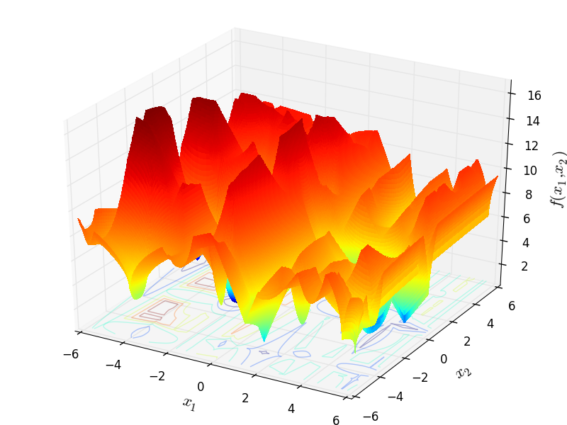
I have compared the results of the original Python code and the ones due to my re-implementation and they are exactly the same: this is easy to see by comparing the figure in the GitHub page above in the paper above with Figure 5.1 below.

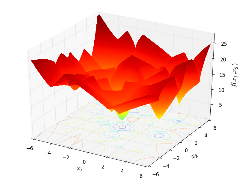
Figure 5.1: A two-dimensional GOTPY function with 10 local minima

Methodology¶

The derivation of the test functions in the GOTPY benchmark suite is fairly straightforward. Although I have no idea where the mathematical methodology comes from - it is not clear from any source - the formulation of the objective function is relatively simple. Assuming we define the following parameters:

The dimensionality $N$ of the problem
The total number of extrema (local and global), as $n$
A list of “steepness” coefficients $a (n \times N)$ . The higher the values, the faster the function decreases / increases and the narrower the area of the minimum
A list of coordinates for the minima, $c (n \times N)$
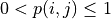A list of degrees of “smoothness” around the each minimum $p (n \times N)$ , if $0 < p(i, j) \leq 1$ the function at the minimum point will be angular
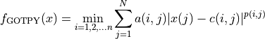
A list of function values, one per minima, $b (n)$

Then the overall expression for any objective function in the GOTPY test suite is:

$f_{\textrm{GOTPY}}(x) = \min_{i=1, 2, ... n} \sum_{j=1}^{N}a(i,j) \lvert x(j)-c(i,j) \rvert^{p(i, j)}$

Since there are quite a few free parameters that we cn change to generate very different benchmark functions, my approach for this test suite has ben the following:

The number of dimensions ranges from $N = 2$ to $N = 5$
The generator creates a total of 100 test function per dimension
The specifications for the parameters of the test generator are as follows:
- The total number of minima is a random integer between 10 and 200
- The coordinates of the aforementioned minima are randomly sampled (uniformly) in the function domain, which I have arbitrarily set at $lb = -6$ and $ub = 6$
- The value of the global minimum is always $f_{opt} = 0.5$ , with the other minima having a function value randomly distributed (uniformly) and sampled to be $f_{opt} + 10 \cdot rand()$
- The smoothing coefficients are randomly uniformly distributed between 0 and 3
- The steepness coefficients are randomly uniformly distributed between 0 and 10

With these settings in mind, I have generated 400 test functions (100 per dimension) from the GOTPY benchmark suite. A few examples of 2D benchmark functions created with the GOTPY generator can be seen in Figure 5.2.

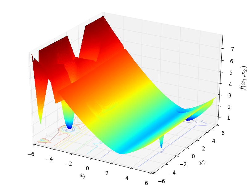
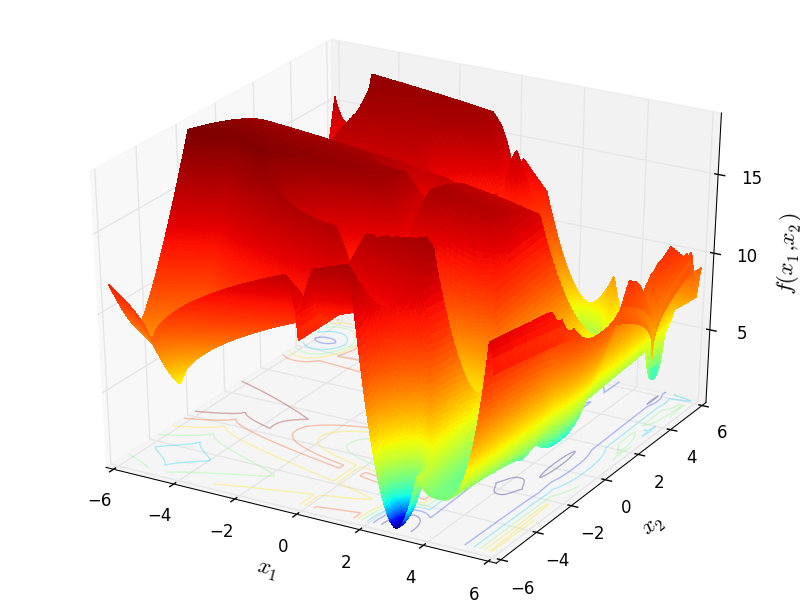
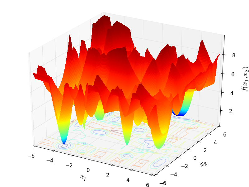
GOTPY Function 1	GOTPY Function 3	GOTPY Function 4
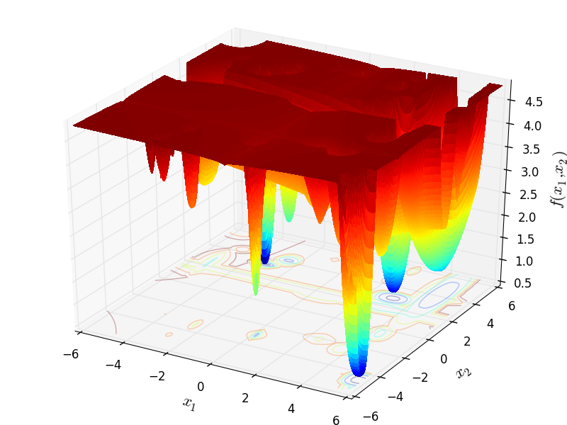
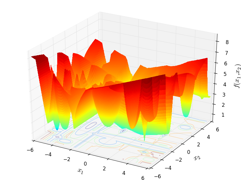
GOTPY Function 7	GOTPY Function 9	GOTPY Function 10

General Solvers Performances¶

Table 5.1 below shows the overall success of all Global Optimization algorithms, considering every benchmark function, for a maximum allowable budget of $NF = 2,000$ .

The table an picture show that the GOTPY benchmark suite is a very hard test suite, as the best solver (DIRECT) only manages to find the global minimum in 23% of the cases, followed at a distance by SHGO and by MCS.

Note

The reported number of functions evaluations refers to successful optimizations only.

**Table 5.1**: Solvers performances on the GOTPY benchmark suite at NF = 2,000
Optimization Method	Overall Success (%)	Functions Evaluations
AMPGO	7.50%	834
BasinHopping	3.25%	547
BiteOpt	11.75%	758
CMA-ES	3.00%	926
CRS2	9.25%	834
DE	6.25%	1,195
DIRECT	23.00%	665
DualAnnealing	8.75%	499
LeapFrog	6.50%	559
MCS	17.50%	878
PSWARM	4.25%	1,242
SCE	7.75%	696
SHGO	18.00%	687

These results are also depicted in Figure 5.3, which shows that DIRECT is the better-performing optimization algorithm, followed by SHGO and MCS.

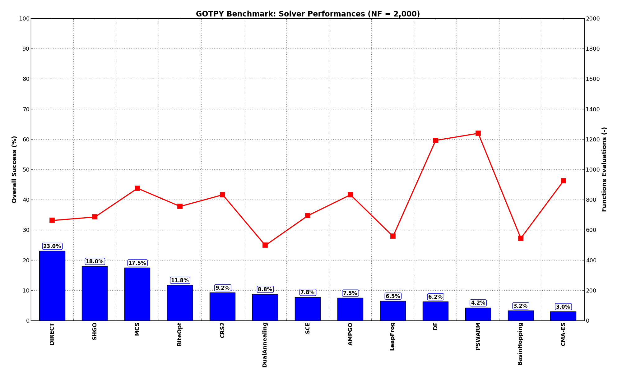
Optimization algorithms performances on the GOTPY test suite at :math:`NF = 2,000`

Figure 5.3: Optimization algorithms performances on the GOTPY test suite at $NF = 2,000$

Pushing the available budget to a very generous $NF = 10,000$ , the results show MCS taking the lead on other solvers (about 18% more problems solved compared to the second best, DIRECT and SHGO). The results are also shown visually in Figure 5.4.

**Table 5.2**: Solvers performances on the GOTPY benchmark suite at NF = 10,000
Optimization Method	Overall Success (%)	Functions Evaluations
AMPGO	25.50%	3,945
BasinHopping	5.00%	2,687
BiteOpt	14.75%	1,539
CMA-ES	6.75%	2,862
CRS2	14.25%	1,856
DE	14.25%	3,466
DIRECT	26.75%	1,204
DualAnnealing	10.50%	936
LeapFrog	6.50%	559
MCS	43.50%	3,219
PSWARM	10.75%	2,147
SCE	10.00%	1,889
SHGO	26.50%	1,970

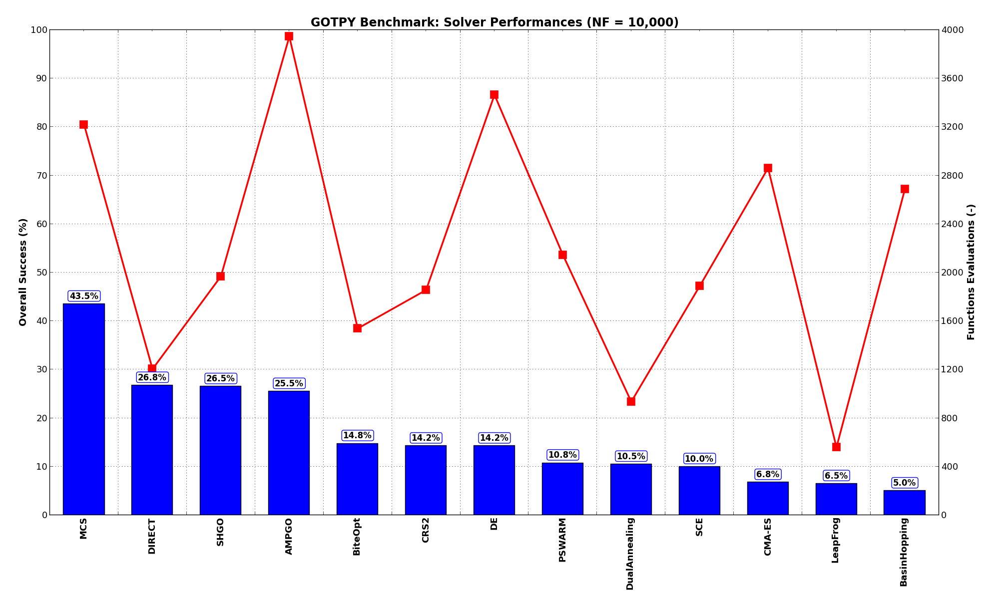
Optimization algorithms performances on the GOTPY test suite at :math:`NF = 10,000`

Figure 5.4: Optimization algorithms performances on the GOTPY test suite at $NF = 10,000$

None of the solver is able to solve at least 50% of th problems, even at a very high budget of function evaluations. Interesting to note the jump of AMPGO, going from 7% success rate to more than 25% when $NF = 10,000$ .

Sensitivities on Functions Evaluations Budget¶

It is also interesting to analyze the success of an optimization algorithm based on the fraction (or percentage) of problems solved given a fixed number of allowed function evaluations, let’s say 100, 200, 300,... 2000, 5000, 10000.

In order to do that, we can present the results using two different types of visualizations. The first one is some sort of “small multiples” in which each solver gets an individual subplot showing the improvement in the number of solved problems as a function of the available number of function evaluations - on top of a background set of grey, semi-transparent lines showing all the other solvers performances.

This visual gives an indication of how good/bad is a solver compared to all the others as function of the budget available. Results are shown in Figure 5.5.

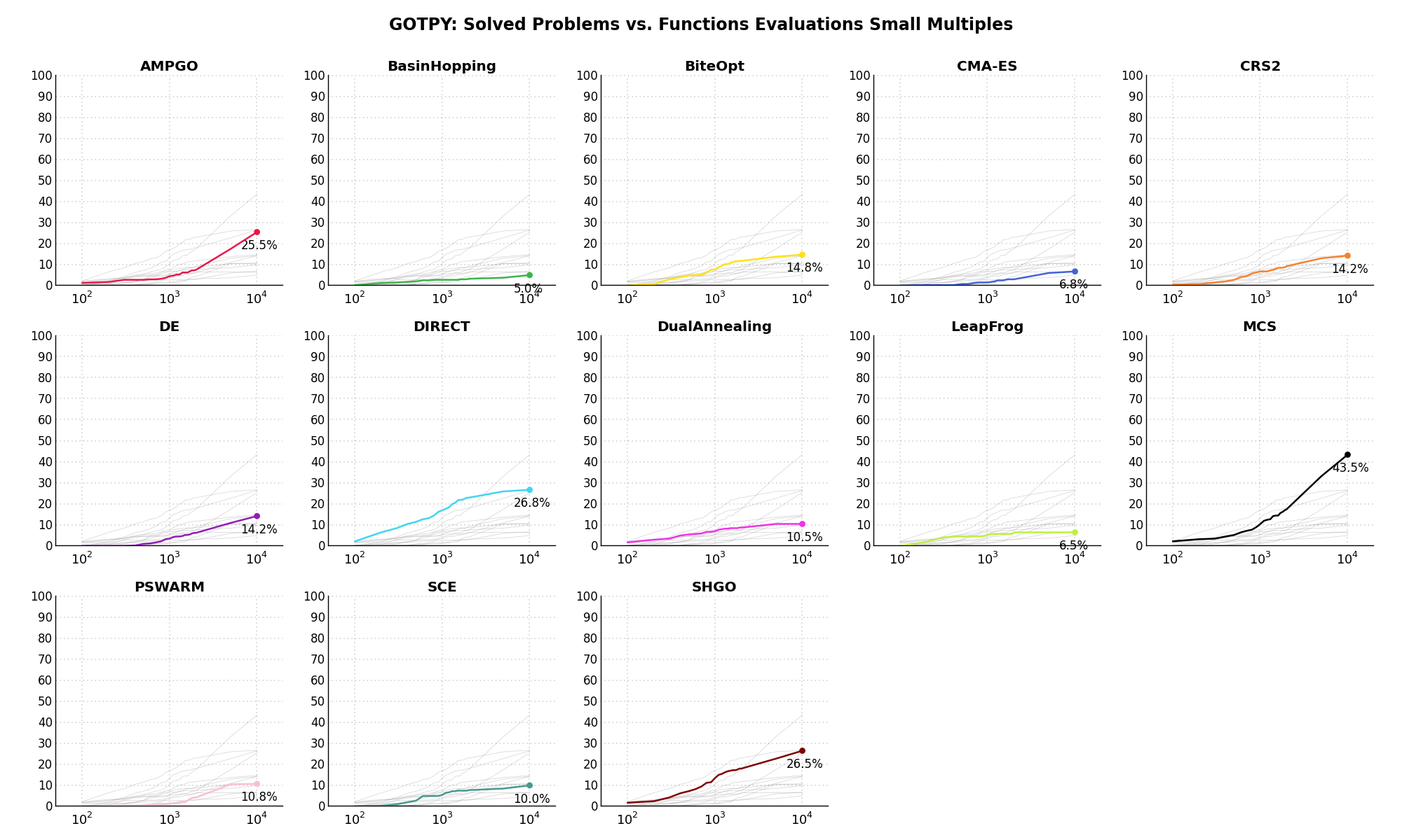
Figure 5.5: Percentage of problems solved given a fixed number of function evaluations on the GOTPY test suite

The second type of visualization is sometimes referred as “Slopegraph” and there are many variants on the plot layout and appearance that we can implement. The version shown in Figure 5.6 aggregates all the solvers together, so it is easier to spot when a solver overtakes another or the overall performance of an algorithm while the available budget of function evaluations changes.

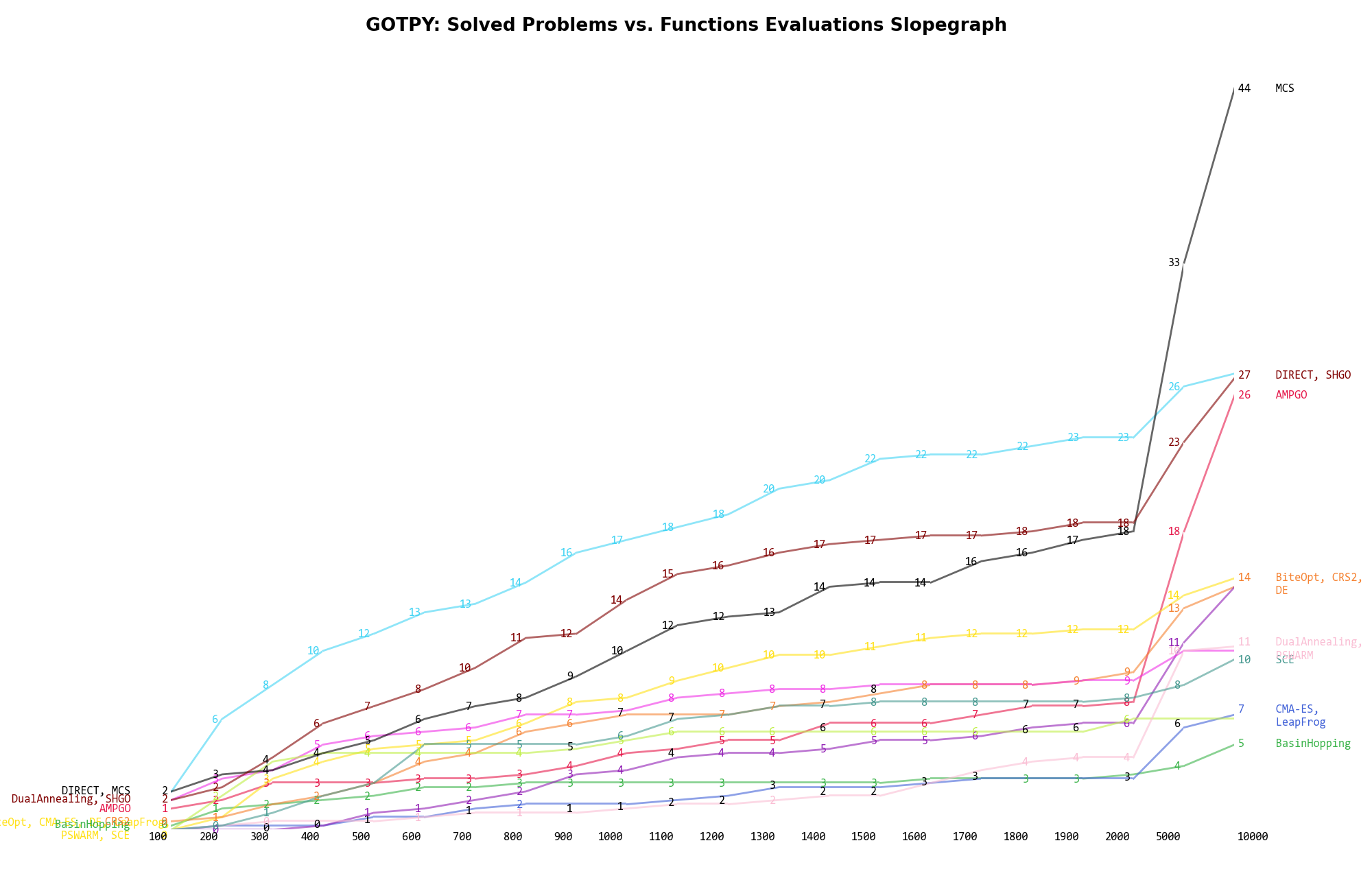
Figure 5.6: Percentage of problems solved given a fixed number of function evaluations on the GOTPY test suite

A few obvious conclusions we can draw from these pictures are:

For this specific benchmark test suite, if you have a very limited budget in terms of function evaluations, then the DIRECT optimizer is a very good first choice - and it is actually the best choice all the way until the available budget becomes very large ( $NF \geq 5,000$ ).
Only a few solvers appear to benefit from the generous function evaluations limits of $NF = 5,000$ and $NF = 10,000$ : specifically, very good improvements can be seen for MCS, AMPGO, SHGO and somewhat less pronounced for DE
None of the solve shines at any level of budget.

Dimensionality Effects¶

Since I used the GOTPY test suite to generate test functions with dimensionality ranging from 2 to 5, it is interesting to take a look at the solvers performances as a function of the problem dimensionality. Of course, in general it is to be expected that for larger dimensions less problems are going to be solved - although it is not always necessarily so as it also depends on the function being generated. Results are shown in Table 5.3 .

**Table 5.3**: Dimensionality effects on the GOTPY benchmark suite at NF = 2,000
Solver	N = 2	N = 3	N = 4	N = 5	Overall
AMPGO	15.0	8.0	3.0	4.0	7.5
BasinHopping	8.0	3.0	2.0	0.0	3.2
BiteOpt	22.0	14.0	6.0	5.0	11.8
CMA-ES	8.0	2.0	2.0	0.0	3.0
CRS2	27.0	6.0	4.0	0.0	9.2
DE	22.0	3.0	0.0	0.0	6.2
DIRECT	53.0	18.0	13.0	8.0	23.0
DualAnnealing	27.0	6.0	2.0	0.0	8.8
LeapFrog	14.0	6.0	3.0	3.0	6.5
MCS	46.0	17.0	3.0	4.0	17.5
PSWARM	16.0	1.0	0.0	0.0	4.2
SCE	24.0	3.0	3.0	1.0	7.8
SHGO	52.0	15.0	3.0	2.0	18.0

Figure 5.7 shows the same results in a visual way.

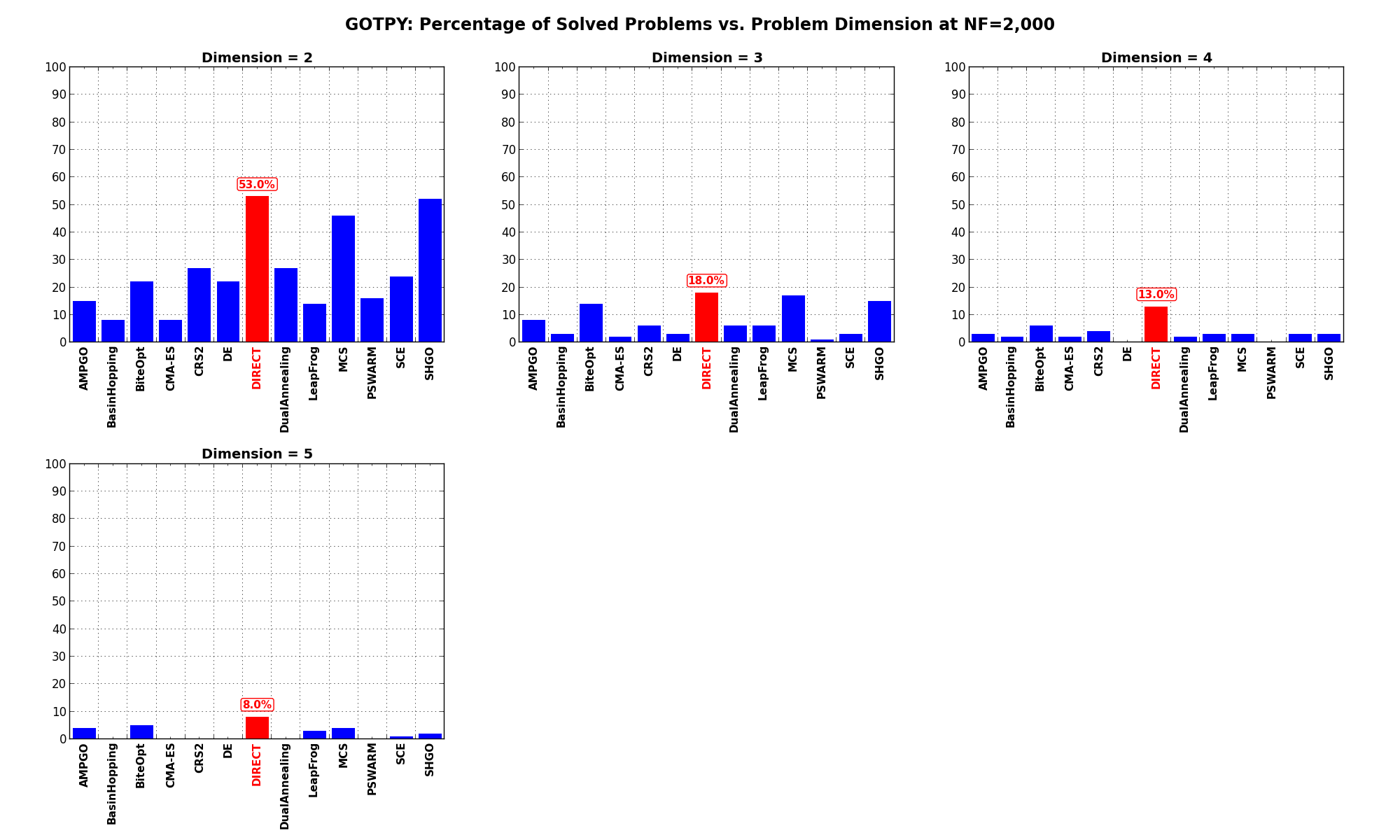
Percentage of problems solved as a function of problem dimension at :math:`NF = 2,000`

Figure 5.7: Percentage of problems solved as a function of problem dimension for the GOTPY test suite at $NF = 2,000$

What we can infer from the table and the figure is that, for lower dimensionality problems ( $NF \leq 3$ ), the DIRECT and SHGO solvers are extremely close in terms of number of problems solved, followed at a distance by MCS. For higher dimensionality problems ( $N > 3$ ), only the DIRECT optimization algorithm seems to deliver any meaningful result - although not exactly spectacular.

Pushing the available budget to a very generous $NF = 10,000$ , the results show MCS solving more problems than any other solver until $NF = 5$ , in which case it is slightly overtaken by AMPGO. For lower dimensionality problems, MCS is tailed at a significant distance by SHGO and DIRECT.

The results for the benchmarks at $NF = 10,000$ are displayed in Table 5.4 and Figure 5.8.

**Table 5.4**: Dimensionality effects on the GOTPY benchmark suite at NF = 10,000
Solver	N = 2	N = 3	N = 4	N = 5	Overall
AMPGO	45.0	27.0	14.0	16.0	25.5
BasinHopping	12.0	5.0	3.0	0.0	5.0
BiteOpt	31.0	15.0	6.0	7.0	14.8
CMA-ES	13.0	9.0	4.0	1.0	6.8
CRS2	28.0	11.0	14.0	4.0	14.2
DE	23.0	13.0	16.0	5.0	14.2
DIRECT	59.0	24.0	16.0	8.0	26.8
DualAnnealing	31.0	8.0	3.0	0.0	10.5
LeapFrog	14.0	6.0	3.0	3.0	6.5
MCS	74.0	58.0	27.0	15.0	43.5
PSWARM	32.0	9.0	2.0	0.0	10.8
SCE	26.0	7.0	6.0	1.0	10.0
SHGO	63.0	30.0	11.0	2.0	26.5

Figure 5.8 shows the same results in a visual way.

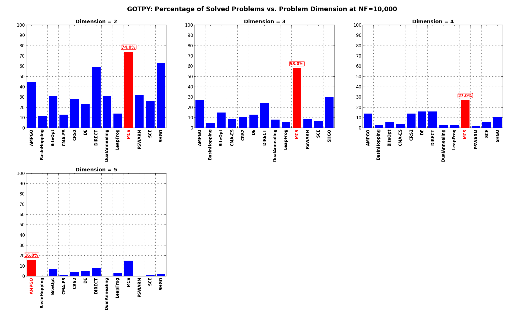
Percentage of problems solved as a function of problem dimension at :math:`NF = 10,000`

Figure 5.8: Percentage of problems solved as a function of problem dimension for the GOTPY test suite at $NF = 10,000$

GOTPY¶

Methodology¶

General Solvers Performances¶

Sensitivities on Functions Evaluations Budget¶

Dimensionality Effects¶

Table Of Contents

Previous topic

Next topic

This Page

Navigation

GOTPY¶

Methodology¶

General Solvers Performances¶

Sensitivities on Functions Evaluations Budget¶

Dimensionality Effects¶

Table Of Contents

Previous topic

Next topic

This Page

Quick search

Navigation