MMTFG¶

F_opt Known	X_opt Known	Difficulty
Yes	Yes	Easy

The MMTFG test function generator of global optimization test functions is almost as famous as the GKLS one. It is described in the paper A framework for generating tunable test functions for multimodal optimization. I have taken the original C code (available at http://www.ronkkonen.com/generator/ ), and I have instructed the benchmark runner (that is written in Python) to communicate with the C driver via input files - the default for the MMTFG generator, as my Cython skills were not good enough to wrap the code as it is.

The acronym MMTFG obviously stands for Multi-Modal Test Function Generator, as the article above describes it.

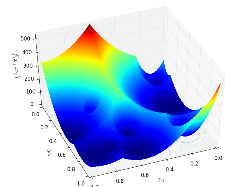
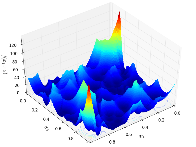
Even though there are no code conversions involved, I still like to check that things add up correctly while using a test functions generator. I then have compared the results of the original C code and of my bridge to it ad they are exactly the same: this is easy to see by comparing Figure 2 (a) and Figure 2 (b) in the paper above with Figure 4.1 below. Thr first picture shows a MMTFG quadratic family function from a two-dimensional test functions with 10 spherical, global minima. The second figure has 10 global and 100 local rotated ellipsoidal minima such that the local minima points have fitness value in range $[-0.95,-0.15]$ . Globally optimal value is always -1.

MMTFG Function 1

MMTFG Function 2

Methodology¶

The MMTFG generator can be used to generate multimodal test functions for minimization, tunable with parameters to allow generation of landscape characteristics that are specifically designed for evaluating multimodal optimization algorithms by their ability to locate multiple optima. At the moment, three families of functions exist, but the generator is easily expandable and new families may be added in future. The current families are cosine, quadratic and common families.

The cosine family samples two cosine curves together, of which one defines global minima and another adds local minima. The basic internal structure is regular: all minima are of similar size and shape and located in rows of similar distance from each other. The function family is defined by:

$f_{cos}(\overrightarrow{y}) = \frac{\sum_{i=1}^{D}-\cos((G_i-1)2\pi y_i) - \alpha \times \cos((G_i-1)2 \pi L_iy_i)}{2D}$

where $\overrightarrow{y} \in [0, 1]^D$ , $D$ is the dimensionality, the parameters $\overrightarrow{G} = (G_1, G_2, ..., G_D)$ and $\overrightarrow{L} = (L_1, L_2, ..., L_D)$ are vectors of positive integers which define the number of global and local minima for each dimension, and $\alpha \in (0, 1]$ defines the amplitude of the sampling function (depth of the local minima). The generator allows the function to be rotated to a random angle and use Bezier curves to stretch each dimension independently to decrease the regularity.

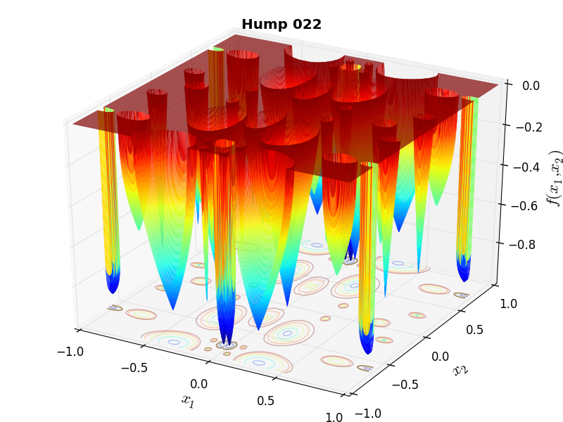
The quadratic family can be used to generate completely irregular landscapes. The function is created by combining several minima generated independently. They are described as a $D$ dimensional general quadratic form, where a symmetric matrix $C$ defines the shape of each minimum. The functions in quadratic family need not be stretched or rotated, because no additional benefit would be gained by doing that to an already irregular function. However, axis-aligned minima may be randomly rotated by rotating the matrix $C$ with a matrix $\mathbf{O} = [\mathbf{\overrightarrow{o_1}}, ..., \mathbf{\overrightarrow{o_D}}]$ is a randomly generated angle preserving orthogonal linear transformation such as:

$\mathbf{B} = \mathbf{O}\mathbf{C}\mathbf{O^T}$

The functions in the quadratic family are then calculated by:

$f_{quad}(\overrightarrow{x}) = \min_{i=1, 2, ... q} ((\overrightarrow{x} - \overrightarrow{p_i})^T \mathbf{B_i^{-1}} (\overrightarrow{x} - \overrightarrow{p_i}) + \nu_i)$

where $\overrightarrow{x} \in [0, 1]^D$ , $\overrightarrow{p_i}$ defines the location and $\nu_i$ the fitness value of a minimum point for the i’th minimum. $q$ is the number of minima.

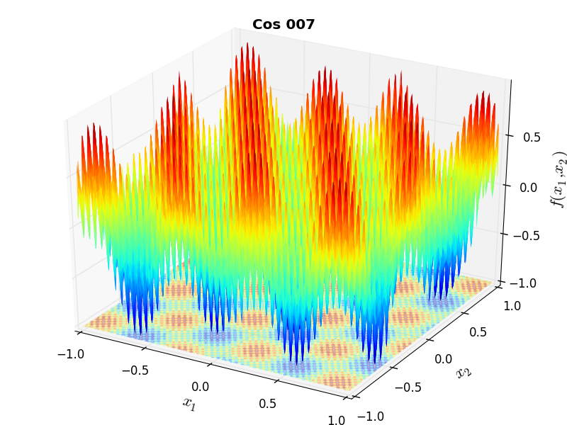
The hump family implements the generic hump functions family proposed by Singh and Deb (2006). Like the quadratic family, the hump functions allow irregular landscapes to be generated and the number of minima to be defined independently of the dimensionality. The placement of minima is chosen randomly. Each minimum is defined by:

$f_{hump}(\overrightarrow{y}) = \begin{cases} h_i\left[1 - \left ( \frac{d(\overrightarrow{y}, i)}{r_i} \right )^{\alpha_i} \right ], & \textrm{ if } d(\overrightarrow{y}, i) \leq r_i \\ 0, & \textrm{ otherwise } \end{cases}$

where $\overrightarrow{y} \in [0, 1]^D$ , $h_i$ is the value of the i th minimum, $d(\overrightarrow{y}, i)$ is the Euclidean distance between $\overrightarrow{y}$ and the center of the i th minimum, 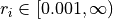$r_i \in [0.001, \infty)$ defines the basin radius and $\alpha \in [0.001, 1]$ the shape of the i th minimum slope.

My approach in building the test functions using the MMTFG generator has been family dependent, and in particular:

For all families, the number of dimensions ranges from 2 to 4
For the cosine family:
- 3 possible values for the number of global optima, randomly chosen between 2 and 8
- 3 possible values for the number of local optima, randomly chosen between 2 and 18
- 3 possible values for the amplitude of the sampling function (depth of local minima), randomly chosen between 0.5 and 0.99
- Whether or not to rotate the test function
- Whether or not to use Bezier curves to stretch each dimension independently to decrease the regularity.
For the quadratic family:
- 2 possible values for the number of global optima, randomly chosen between 1 and 8
- 3 possible values for the number of local optima, either 0, 5 or 10
- 3 possible values for the shape of the generated optima (both local and global)
- 5 possible values for the minimum euclidean distance between two global optima, randomly chosen but respecting the constraints built in the test function generator
- 2 possible values for the lower and upper limit for the shape of the global optima, randomly chosen but respecting the constraints built in the test function generator
- 2 possible values for the lower and upper limit for the shape of the local optima, randomly chosen but respecting the constraints built in the test function generator
For the hump family:
- 3 possible values for the number of global optima, either 1, 3, or 5
- 2 possible values for the number of local optima, either 0, 10
- 3 possible values for the local optima values, linearly spaced between -0.95 and -0.02
- 2 possible values for the range for hump radii, either 0.01 or 0.95
- 3 possible values for the range for hump shape parameter, linearly spaced between 0.01 and 0.95
- Whether or not to rotate the test function
- Whether or not to use Bezier curves to stretch each dimension independently to decrease the regularity.

Armed with all these combinations - and please keep in mind that some combinations, especially in the quadratic family, are invalid due to internal constraints in the test function generator - I have generated a total of 981 benchmark functions divided as presented in Table 4.1:

**Table 4.1**: Number of benchmark functions in the MMTFG test suite
Family	N = 2	N = 3	N = 4	Total
Cos	108	108	108	324
Hump	96	96	96	288
Quad	108	126	135	369
Total	312	330	339	981

A few examples of 2D benchmark functions created with the MMTFG generator can be seen in Figure 4.2.

MMTFG Cosine 7	MMTFG Hump 22	MMTFG Quad 17
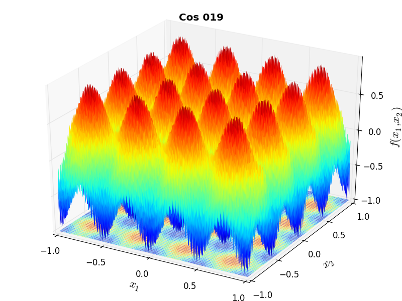
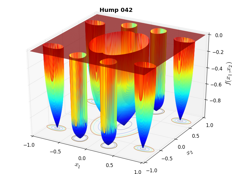
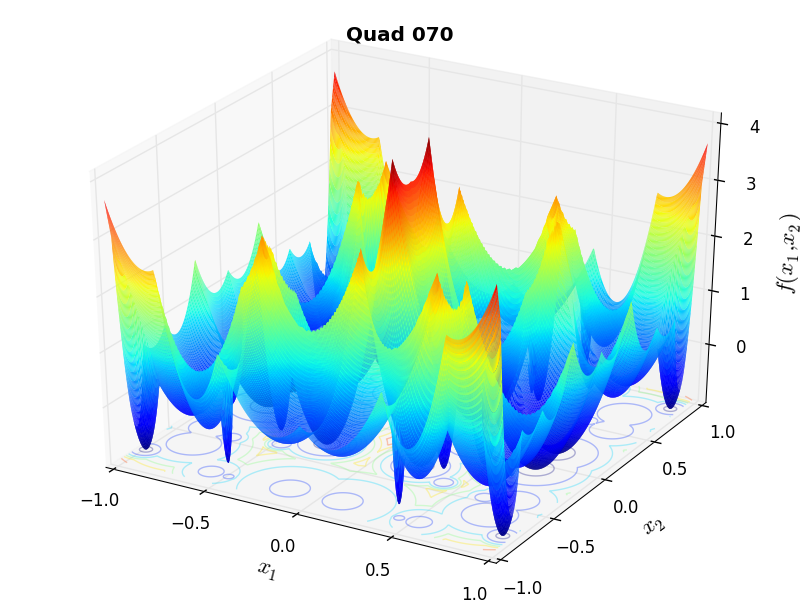
MMTFG Cosine 19	MMTFG Hump 42	MMTFG Quad 70

General Solvers Performances¶

Table 4.2 below shows the overall success of all Global Optimization algorithms, considering every benchmark function, for a maximum allowable budget of $NF = 2,000$ .

As we can see - and in contrast with the GKLS and GlobOpt test function generators - the level of difficulty of the MMTFG test suite is much lower, as the best solver ( MCS) solves up to 77% of all the problems with less than 300 function evaluations. Second comes the BiteOpt algorithm, but many of the SciPy solvers are up there too - BasinHopping, DualAnnealing and SHGO provide excellent performances on this test suite.

Note

The reported number of functions evaluations refers to successful optimizations only.

**Table 4.2**: Solvers performances on the MMTFG benchmark suite at NF = 2,000
Optimization Method	Overall Success (%)	Functions Evaluations
AMPGO	60.24%	461
BasinHopping	72.07%	319
BiteOpt	72.27%	515
CMA-ES	52.19%	570
CRS2	49.85%	1,007
DE	32.93%	1,396
DIRECT	59.43%	419
DualAnnealing	66.97%	313
LeapFrog	43.93%	278
MCS	77.06%	287
PSWARM	19.57%	890
SCE	24.57%	958
SHGO	69.22%	295

These results are also depicted in Figure 4.3, which shows that MCS is the better-performing optimization algorithm, followed by BiteOpt and BasinHopping.

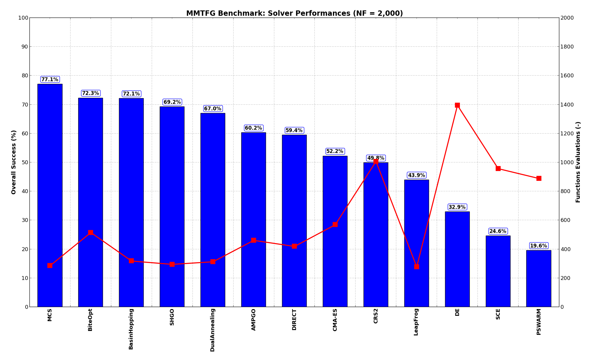
Optimization algorithms performances on the MMTFG test suite at :math:`NF = 2,000`

Figure 4.3: Optimization algorithms performances on the MMTFG test suite at $NF = 2,000$

Pushing the available budget to a very generous 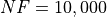$NF = 10,000$ , the results show MCS taking the lead on other solvers (about 6% more problems solved compared to the second best, BiteOpt). The results are also shown visually in Figure 4.4.

**Table 4.3**: Solvers performances on the MMTFG benchmark suite at NF = 10,000
Optimization Method	Overall Success (%)	Functions Evaluations
AMPGO	75.84%	1,359
BasinHopping	77.68%	518
BiteOpt	78.90%	887
CMA-ES	66.77%	1,449
CRS2	61.06%	1,422
DE	71.97%	2,880
DIRECT	64.42%	746
DualAnnealing	71.25%	473
LeapFrog	43.93%	278
MCS	85.52%	726
PSWARM	67.69%	2,454
SCE	35.47%	2,018
SHGO	78.70%	679

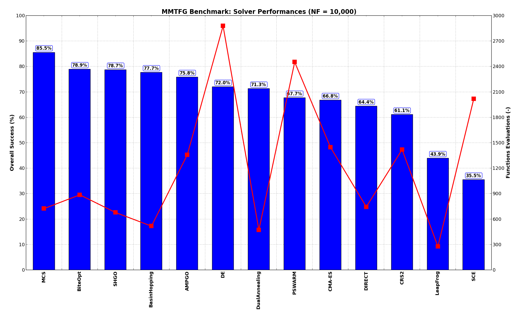
Optimization algorithms performances on the MMTFG test suite at :math:`NF = 10,000`

Figure 4.4: Optimization algorithms performances on the MMTFG test suite at $NF = 10,000$

All the solvers except for LeapFrog and SCE are able to solve more than 60% of the problems if given a generous budget as we did above at $NF = 10,000$ .

Sensitivities on Functions Evaluations Budget¶

It is also interesting to analyze the success of an optimization algorithm based on the fraction (or percentage) of problems solved given a fixed number of allowed function evaluations, let’s say 100, 200, 300,... 2000, 5000, 10000.

In order to do that, we can present the results using two different types of visualizations. The first one is some sort of “small multiples” in which each solver gets an individual subplot showing the improvement in the number of solved problems as a function of the available number of function evaluations - on top of a background set of grey, semi-transparent lines showing all the other solvers performances.

This visual gives an indication of how good/bad is a solver compared to all the others as function of the budget available. Results are shown in Figure 4.5.

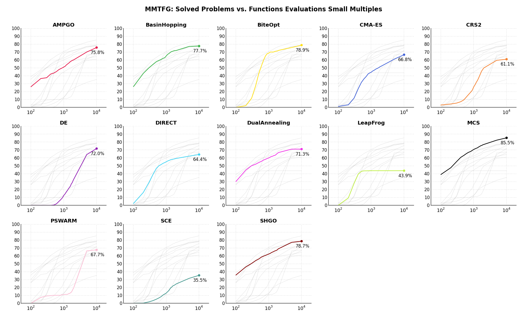
Figure 4.5: Percentage of problems solved given a fixed number of function evaluations on the MMTFG test suite

The second type of visualization is sometimes referred as “Slopegraph” and there are many variants on the plot layout and appearance that we can implement. The version shown in Figure 4.6 aggregates all the solvers together, so it is easier to spot when a solver overtakes another or the overall performance of an algorithm while the available budget of function evaluations changes.

Figure 4.6: Percentage of problems solved given a fixed number of function evaluations on the MMTFG test suite

A few obvious conclusions we can draw from these pictures are:

For this specific benchmark test suite, if you have a very limited budget in terms of function evaluations, then MCS is a very good first choice. Following very close by, any of the SciPy Global Optimization Algorithms is going to do a fine job, solving between 60% and 70% of all problems with less than $NF = 1,000$ function evaluations.....
There is a phenomenal ramp up in performances - again - for PSWARM between $NF = 2,000$ and $NF = 10,000$ , and a very similar argument can be made for DE.
The performances of the SCE algorithm are puzzling to say the least, while LeapFrog never recovers even when given extremely generous budgets.

Dimensionality Effects¶

Since I used the MMTFG test suite to generate test functions with dimensionality ranging from 2 to 4, it is interesting to take a look at the solvers performances as a function of the problem dimensionality. Of course, in general it is to be expected that for larger dimensions less problems are going to be solved - although it is not always necessarily so as it also depends on the function being generated. Results are shown in Table 4.4 .

**Table 4.4**: Dimensionality effects on the MMTFG benchmark suite at NF = 2,000
Solver	N = 2	N = 3	N = 4	Overall
AMPGO	76.9	63.6	41.6	60.7
BasinHopping	83.3	71.2	62.5	72.4
BiteOpt	84.6	71.5	61.7	72.6
CMA-ES	68.9	50.0	38.9	52.6
CRS2	74.4	50.6	26.5	50.5
DE	77.9	24.2	0.0	34.0
DIRECT	78.2	58.2	43.4	59.9
DualAnnealing	86.9	61.5	54.0	67.5
LeapFrog	57.7	46.4	28.9	44.3
MCS	92.6	76.1	63.7	77.5
PSWARM	33.7	10.6	15.3	19.9
SCE	39.1	18.8	16.8	24.9
SHGO	88.8	68.5	51.9	69.7

Figure 4.7 shows the same results in a visual way.

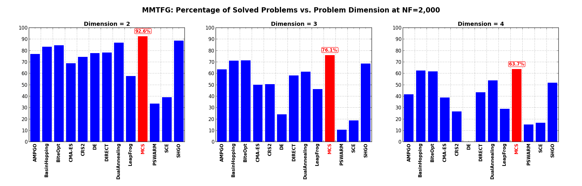
Percentage of problems solved as a function of problem dimension at :math:`NF = 2,000`

Figure 4.7: Percentage of problems solved as a function of problem dimension for the MMTFG test suite at $NF = 2,000$

What we can infer from the table and the figure is that, for lower dimensionality problems ( $NF < 3$ ), MCS, SHGO, BasinHopping and BiteOpt solve the vast majority of problems (90%). For higher dimensionality problems ( $N \geq 3$ ), all those solvers keep a very good performance, although it is to be expected that the number of problems solved decreases with $N$ . A dramatic drop in ability to find global optima can be seen for the DE algorithm, which crashes from 78% success rate at $N = 2$ to 0% success for $N = 4$ .

Pushing the available budget to a very generous $NF = 10,000$ , the results show MCS solving in essence all the problems at low dimensionality ( $N = 2$ ), closely followed by SHGO, BasinHopping and BiteOpt with more than 90% of global minima found. For the highest dimensionality in this test suite ( $N = 4$ ), we can of course observe the resurgence of DE which goes up to 55% success rate.

The results for the benchmarks at $NF = 10,000$ are displayed in Table 4.5 and Figure 4.8.

**Table 4.5**: Dimensionality effects on the MMTFG benchmark suite at NF = 10,000
Solver	N = 2	N = 3	N = 4	Overall
AMPGO	93.3	74.8	60.8	76.3
BasinHopping	90.4	75.8	67.8	78.0
BiteOpt	92.3	77.6	67.8	79.2
CMA-ES	78.8	68.5	54.0	67.1
CRS2	75.0	61.5	47.8	61.4
DE	87.5	74.2	55.5	72.4
DIRECT	87.2	59.7	48.1	65.0
DualAnnealing	89.7	66.1	59.3	71.7
LeapFrog	57.7	46.4	28.9	44.3
MCS	98.7	85.5	73.5	85.9
PSWARM	83.3	62.1	58.7	68.1
SCE	48.1	30.0	29.2	35.8
SHGO	95.5	81.2	60.8	79.2

Figure 4.8 shows the same results in a visual way.

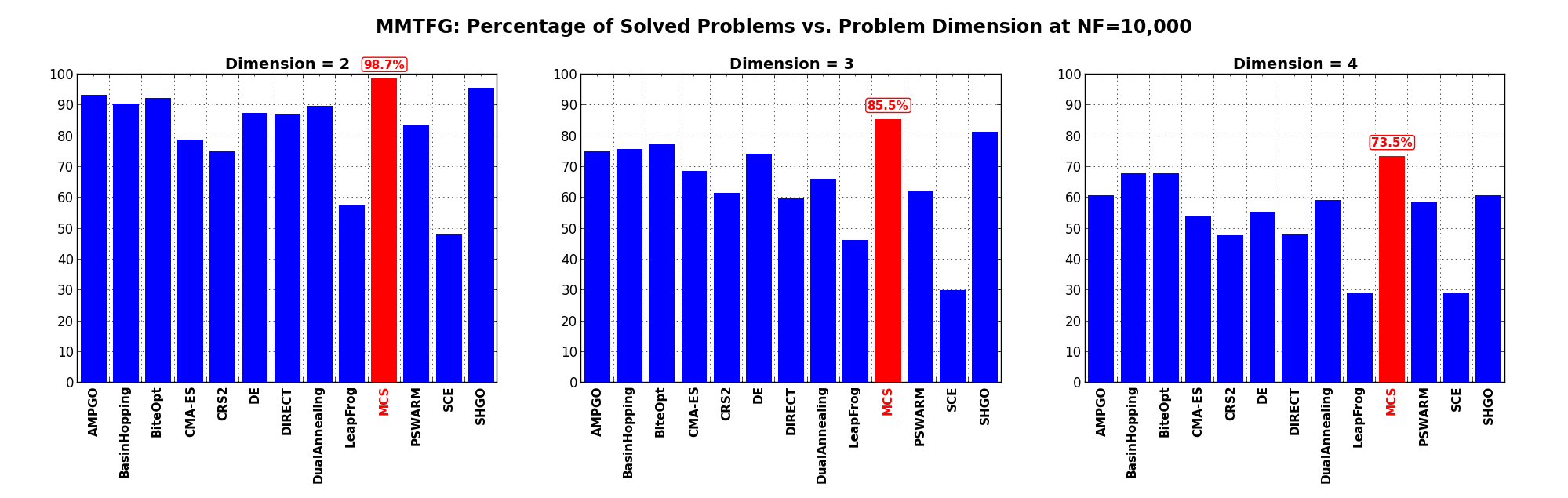
Percentage of problems solved as a function of problem dimension at :math:`NF = 10,000`

Figure 4.8: Percentage of problems solved as a function of problem dimension for the MMTFG test suite at $NF = 10,000$

Family Issues¶

For this specific test suite, it is interesting to see if any particular family of functions is easier or harder to solve compared to the others, across all optimization algorithms. This type of results is shown in Table 4.6 and Table 4.7 below, for $NF = 2,000$ and $NF = 10,000$ maximum budget of function evaluations respectively.

**Table 4.6**: Family effects on the MMTFG benchmark suite at NF = 2,000
Solver	Cosine	Hump	Quadratic	Overall
AMPGO	54.3%	54.9%	69.6%	60.2%
BasinHopping	59.9%	63.2%	89.7%	72.1%
BiteOpt	64.2%	75.0%	77.2%	72.3%
CMA-ES	43.2%	35.1%	73.4%	52.2%
CRS2	44.8%	42.7%	59.9%	49.8%
DE	17.3%	32.6%	46.9%	32.9%
DIRECT	17.3%	75.0%	84.3%	59.4%
DualAnnealing	51.2%	60.8%	85.6%	67.0%
LeapFrog	10.5%	56.2%	63.7%	43.9%
MCS	70.7%	73.6%	85.4%	77.1%
PSWARM	40.7%	0.0%	16.3%	19.6%
SCE	0.0%	38.9%	35.0%	24.6%
SHGO	63.0%	50.7%	89.2%	69.2%
Total	41.3%	50.7%	67.4%	53.9%

**Table 4.7**: Family effects on the MMTFG benchmark suite at NF = 10,000
Solver	Cosine	Hump	Quadratic	Overall
AMPGO	67.6%	71.9%	86.2%	75.8%
BasinHopping	67.0%	69.8%	93.2%	77.7%
BiteOpt	76.5%	78.5%	81.3%	78.9%
CMA-ES	77.2%	38.5%	79.7%	66.8%
CRS2	48.1%	63.5%	70.5%	61.1%
DE	45.7%	81.6%	87.5%	72.0%
DIRECT	25.0%	78.8%	87.8%	64.4%
DualAnnealing	59.6%	63.2%	87.8%	71.3%
LeapFrog	10.5%	56.2%	63.7%	43.9%
MCS	75.3%	84.7%	95.1%	85.5%
PSWARM	56.5%	68.4%	77.0%	67.7%
SCE	0.3%	55.6%	50.7%	35.5%
SHGO	71.6%	64.9%	95.7%	78.7%
Total	52.4%	67.4%	81.2%	67.6%

What seems clear from this tables is that, no matter whether our budget is relatively limited at $NF = 2,000$ or very generous at $NF = 10,000$ , the Cosine family appears to be the toughest set to crack, while the Quadratic family is generally much easier to solve, for almost all the global optimization algorithms considered.

This can also be seen in the heatmap presented in Figure 4.9.

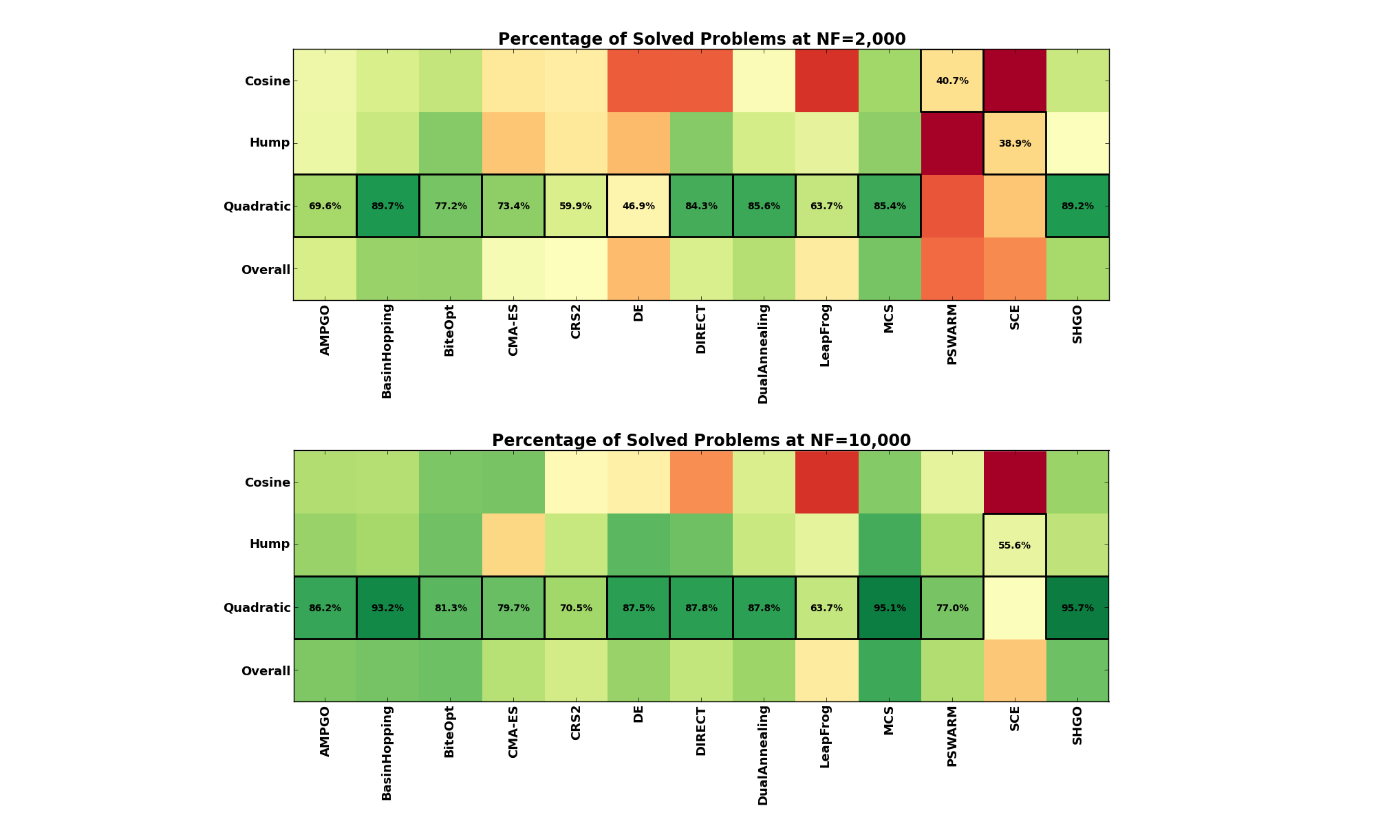
Figure 4.9: Family effects on the MMTFG benchmark suite at $NF = 2,000$ and $NF = 10,000$

MMTFG¶

Methodology¶

General Solvers Performances¶

Sensitivities on Functions Evaluations Budget¶

Dimensionality Effects¶

Family Issues¶

Table Of Contents

Previous topic

Next topic

This Page

Navigation

MMTFG¶

Methodology¶

General Solvers Performances¶

Sensitivities on Functions Evaluations Budget¶

Dimensionality Effects¶

Family Issues¶

Table Of Contents

Previous topic

Next topic

This Page

Quick search

Navigation