Huygens

Fopt Known	Xopt Known	Difficulty
No	No	Medium

The Huygens benchmark is a very fascinating “landscape generator”, with a unique and very characteristic approach in generating test functions for global optimization benchmarks. This particular generator is based on the concept of “fractal functions” and its philosophy is that since many standard functions used for benchmarking are built from a number of elementary mathematical functions, these functions necessarily reduce in detail (or “smooth out”) as you zoom in on the function, meaning that they also smooth out as a solution algorithm converges on a solution.

This has the potential to favour some algorithms that might otherwise not perform so well. In particular, it tips the balance between exploration and exploitation.

The fractal functions, on the other hand, have the property of randomised self-similarity - as the resolution increases the average level of detail remains the same. This avoids many of these biases, and allows the balance between exploration and exploitation in solution functions to be examined more rigorously.

The Huygens generator is described in the paper Benchmarking Evolutionary and Hybrid Algorithms using Randomized Self-Similar Landscapes, and very high level description of fractal functions - together with the code in Java - can be found at the website https://www.cs.bham.ac.uk/research/projects/ecb/displayDataset.php?id=150 .

My original idea was to try and convert the original Java code to Python and NumPy, and that is what I have done as first step. That said, the recursive nature of this benchmark test suite makes Python phenomenally, unbearably slow. I then put all my efforts in writing a Cython version of the Python code, which was about 45% faster (!!!). I then got fed up and I rewrote the whole thing in Fortran, wrapping the resulting f90 modules with f2py.

The overall improvement was stunning, please see Table 6.1 below:

Table 6.1: Simulation speed for the Huygens benchmark in different languages

Language	CPU Time (ms)	Speed up vs. Python
Python	3.1	1.0
Cython	2.2	1.41
Fortran	0.028	111

Of course, my Cython is extremely weak and it is likely that major improvements could be made by an expert - but I had no time to delve into such stuff. I have compared the results of the original Java code and the ones due to my conversion and they are exactly the same: this is easy to see by comparing the example functions in the website linked above with Figure 6.1 below.

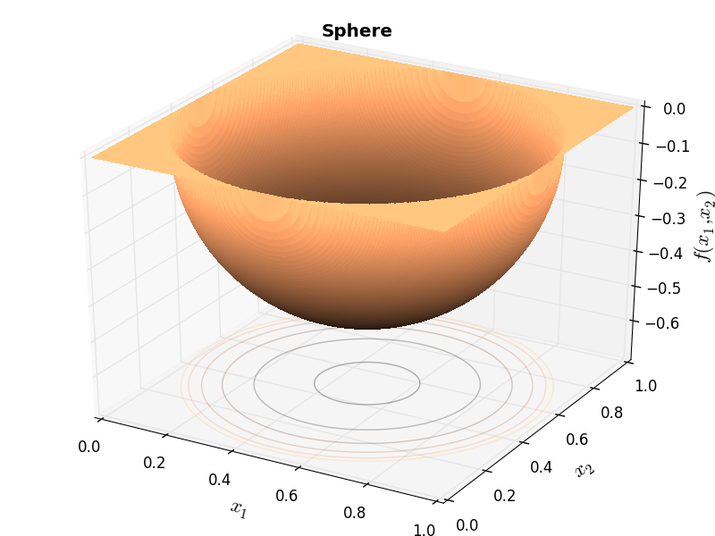
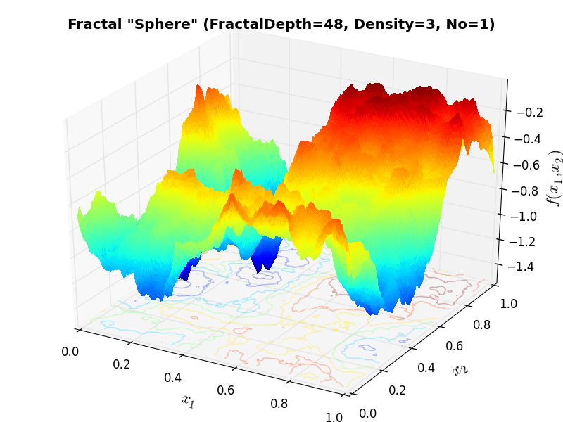
Huygens Unit Function “Sphere”	Huygens Sphere Fractal
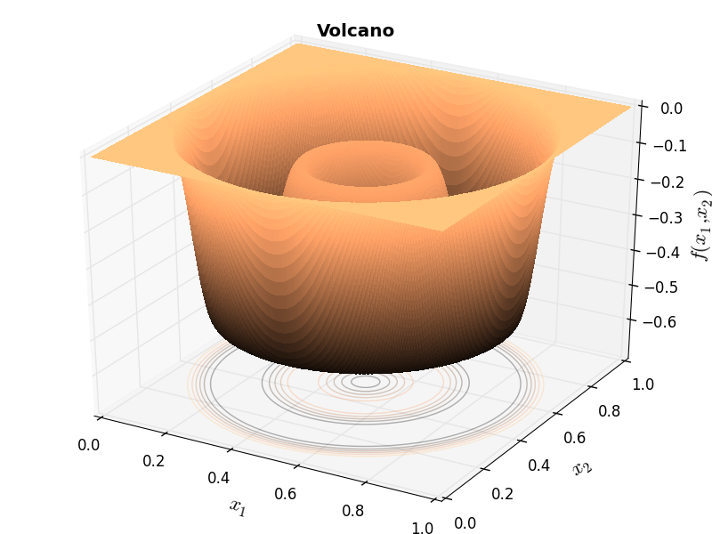
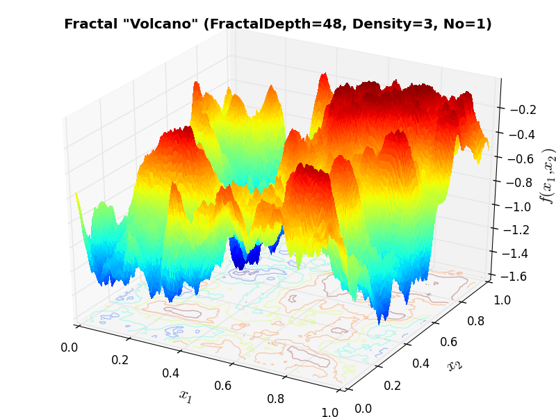
Huygens Unit Function “Volcano”	Huygens Volcano Fractal
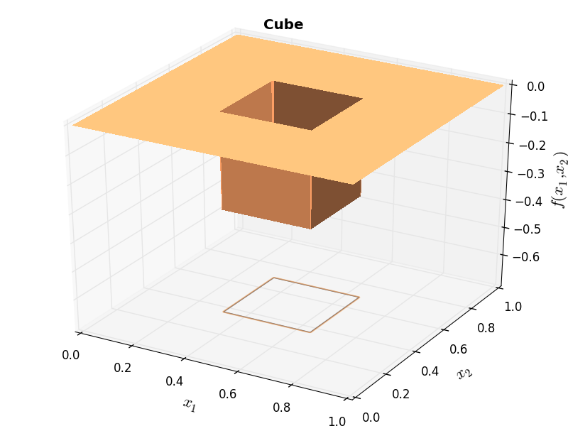
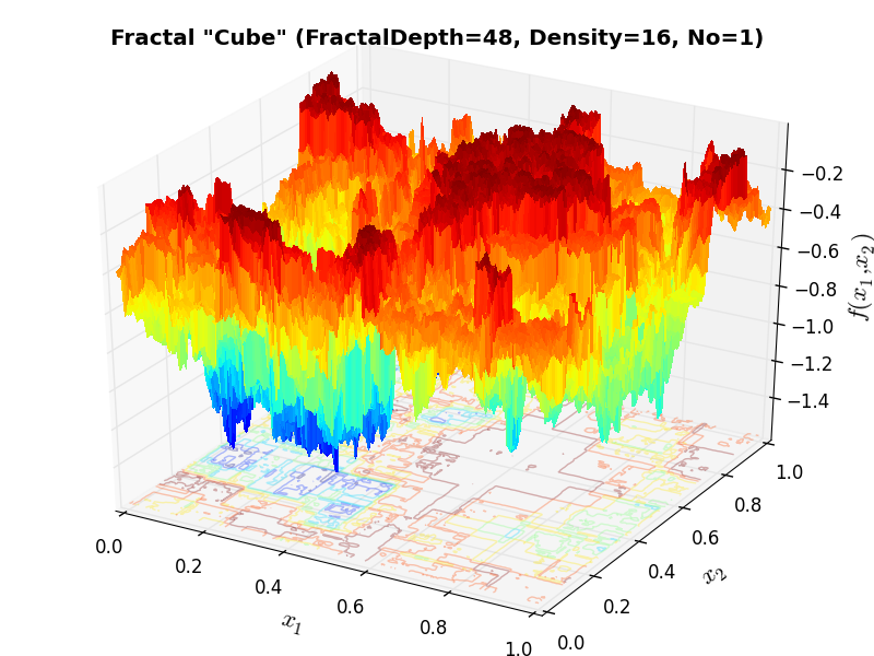
Huygens Unit Function “Cube”	Huygens Cube Fractal

Methodology

The derivation of the test functions in the Huygens benchmark suite is very interesting, as it uses the “Crater Algorithm”: the approach in generating landscapes is based on a (very) simplified model of the natural process of meteors impacting a planetary surface. The assumption is that each surface is initially smooth, and each meteor that impacts it superimposes a crater the size of the bottom half of the meteor. The meteor impacts must be randomly distributed, subject to the constraint that the probability of an impact is related to the meteor size in such as way as to generate self-similarity. The surface “ages” or matures as it receives more and more impacts.

While the x, y positions of craters can be chosen, using random deviates from a uniform probability distribution, the number of meteors of each size must be chosen so as to preserve statistical self-similarity. The average number of craters per order of magnitude is dependent on the age of the landscape.

This is illustrated in Table 6.2 below, with increasing crater numbers with reducing scale, where the average number of craters per order of magnitude square, , determines the age of the landscape

Table 6.2: Number of “craters” in the Huygens benchmark test functions

Scale (or Resolution)	Crater Size Range	Mean Total Number of Craters
...	...	...

Each landscape is uniquely determined by its age (mean number of craters per order of magnitude square) and index (seed).

The Huygens test suite is able to use “seed” test functions (unit functions as displayed above in Figure 6.1, so my approach has been the following:

1. Even though there is a specific Java module named “FastFractal” that you can use to generate test functions with dimensionality greater than , I have elected to use only two-dimensional fractal functions.
2. For each unit function (Cube, Pyramid, Rastrigin2D, Sphere, Volcano), I have considered the “fractal depth” parameter to assume the values 8, 16, 32 and 48, the “fractal density” parameter to be 3, 6, 9, 12, 15, 16 and finally a “seed” parameter varying from 1 to 5. This gives a total of 600 2D objective functions.

One of the main differences between the Huygens benchmark and all the other test suites prior to it is that neither the global optimum position nor the actual minimum value of the objective function is known. So, in order to evaluate the solvers performances in a similar way as done previously, I have elected to follow this approach, for each of the 600 2D fractal functions in the Huygens test suite:

1. Generate a brute-force grid of 2D points between 0 and 1 (the actual bounds). This grid is composed by 1,000,000 points (1,000 x 1,000).
2. Evaluate the objective function at each of these points.
3. After identifying the most promising 1,000 points in the grid (i.e., points for which the function value is lowest), start 3 different local optimization algorithms from each of these points. The algorithms selected for this exercise were a mix of derivative-free and gradient-based approaches (L-BFGS-B, Subplex, Power methods).
4. Out of all these minimizations, the lowest function value obtained becomes the putative “global minimum” for the current fractal functions.

As an example, the effect of the “fractal density” parameter can be seen in Figure 6.3 below.

Figure 6.3: Effect of “fractal density” parameter on a Huygens test function

General Solvers Performances

Table 6.3 below shows the overall success of all Global Optimization algorithms, considering every benchmark function, for a maximum allowable budget of .

The table an picture show that the Huygens benchmark suite is a generally hard test suite, except surprisingly for DIRECT, which manages an excellent 67% overall result, almost twice as good as the closest follower DE.

Note

The reported number of functions evaluations refers to successful optimizations only.

Table 6.3: Solvers performances on the Huygens benchmark suite at NF = 2,000

Optimization Method	Overall Success (%)	Functions Evaluations
AMPGO	13.00%	910
BasinHopping	2.00%	871
BiteOpt	22.50%	707
CMA-ES	8.00%	827
CRS2	22.67%	936
DE	36.50%	1,395
DIRECT	67.00%	733
DualAnnealing	2.83%	906
LeapFrog	6.17%	281
MCS	11.50%	1,030
PSWARM	1.83%	1,610
SCE	14.50%	1,216
SHGO	3.00%	819

These results are also depicted in Figure 6.4, which shows that DIRECT is the better-performing optimization algorithm, followed by DE and BiteOpt.

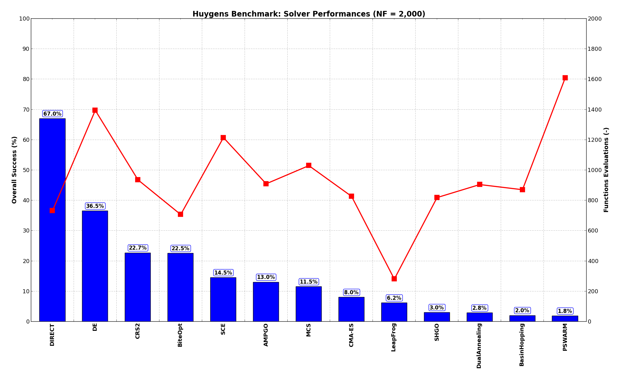
Figure 6.4: Optimization algorithms performances on the Huygens test suite at

Pushing the available budget to a very generous 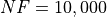, the results show DIRECT still largely outmatching all other optimization algorithms, with almost 75% of the problems solved. AMPGO has a partial comeback, positioning itself on second place. The results are also shown visually in Figure 6.5.

Table 6.4: Solvers performances on the Huygens benchmark suite at NF = 10,000

Optimization Method	Overall Success (%)	Functions Evaluations
AMPGO	40.17%	3,960
BasinHopping	4.50%	2,701
BiteOpt	34.00%	2,129
CMA-ES	22.33%	3,603
CRS2	23.17%	1,020
DE	36.83%	1,407
DIRECT	74.67%	1,109
DualAnnealing	9.00%	2,359
LeapFrog	6.17%	281
MCS	27.67%	3,407
PSWARM	37.50%	3,727
SCE	35.83%	3,176
SHGO	6.00%	3,146

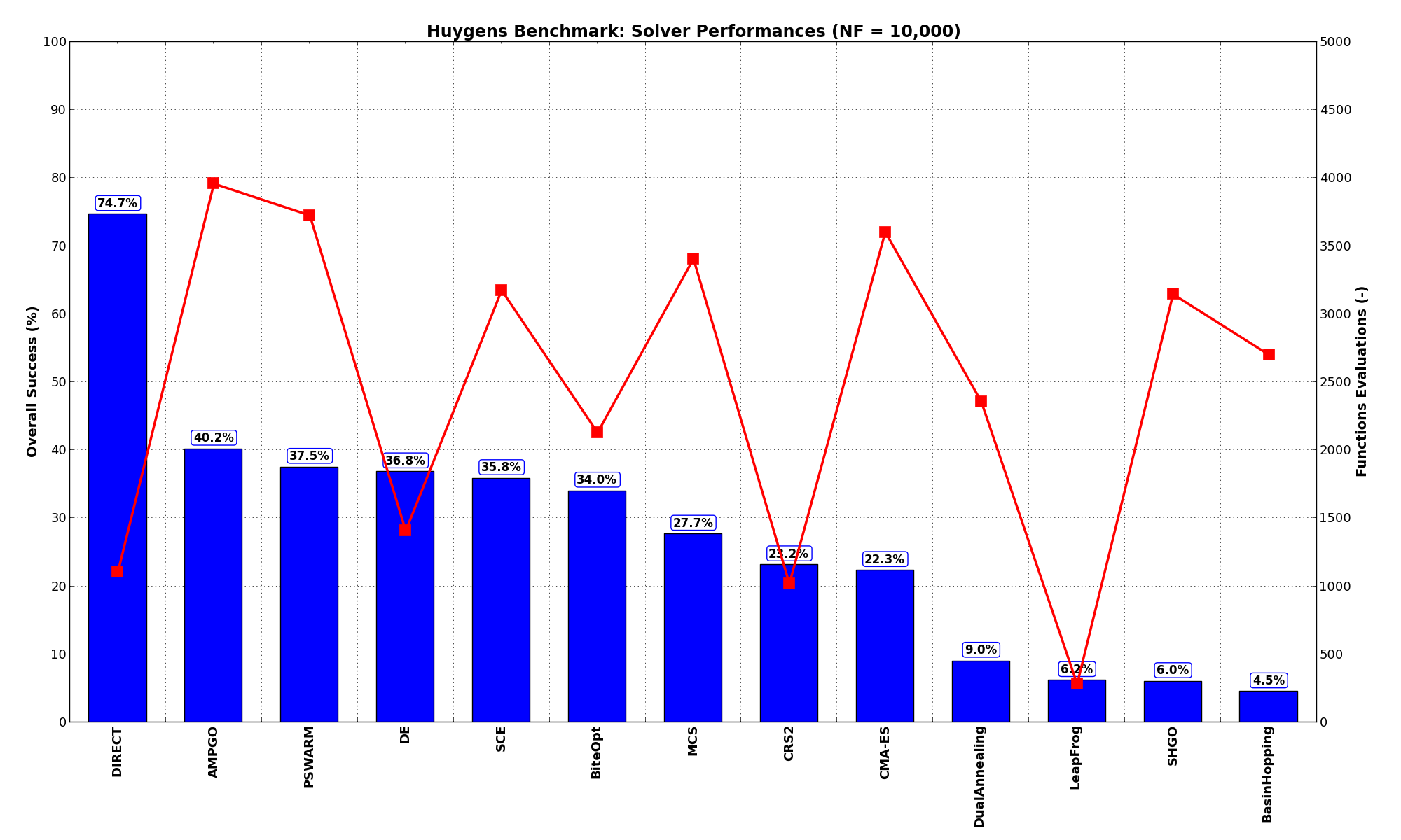
Figure 6.5: Optimization algorithms performances on the Huygens test suite at

I am not clear why DIRECT is so successful in this specific test suite.

Sensitivities on Functions Evaluations Budget

It is also interesting to analyze the success of an optimization algorithm based on the fraction (or percentage) of problems solved given a fixed number of allowed function evaluations, let’s say 100, 200, 300,... 2000, 5000, 10000.

In order to do that, we can present the results using two different types of visualizations. The first one is some sort of “small multiples” in which each solver gets an individual subplot showing the improvement in the number of solved problems as a function of the available number of function evaluations - on top of a background set of grey, semi-transparent lines showing all the other solvers performances.

This visual gives an indication of how good/bad is a solver compared to all the others as function of the budget available. Results are shown in Figure 6.6.

Figure 6.6: Percentage of problems solved given a fixed number of function evaluations on the Huygens test suite

The second type of visualization is sometimes referred as “Slopegraph” and there are many variants on the plot layout and appearance that we can implement. The version shown in Figure 6.7 aggregates all the solvers together, so it is easier to spot when a solver overtakes another or the overall performance of an algorithm while the available budget of function evaluations changes.

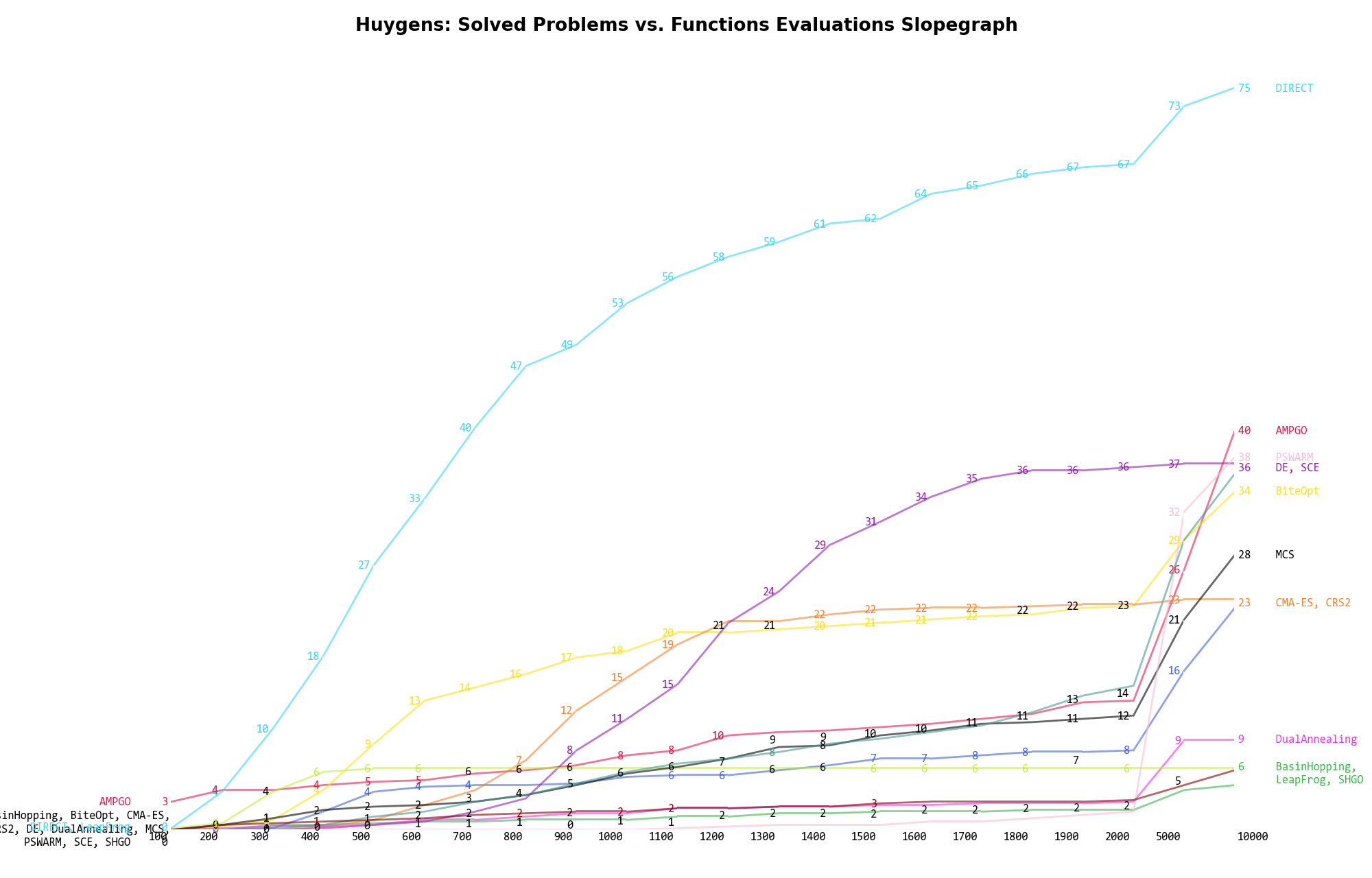
Figure 6.7: Percentage of problems solved given a fixed number of function evaluations on the Huygens test suite

A few obvious conclusions we can draw from these pictures are:

1. For this specific benchmark test suite, none of the solvers achieve satisfactory results except DIRECT.
2. Solvers like AMPGO and PSWARM achieve a very steep improvement in number of problems solved when the limit on number of function evaluations is relaxed to a very high value, but in any case they are far behind of what DIRECT can provide.

Fractal Types

Once the benchmarks were completed, I started wondering whether some of the fractal unit functions may be “easier” to solve compared to others. After all, the unit functions defining those fractals are very different to start with, so we may expect some variability in the ability of any solver to locate a global optimum. Results are shown in Table 6.5 .

Table 6.5: Effect of fractal type on the Huygens benchmark suite at NF = 10,000

Solver	Cube	Pyramid	Rastrigin2D	Sphere	Volcano	Overall
AMPGO	5.8%	67.5%	20.8%	60.0%	46.7%	40.2%
BasinHopping	0.0%	7.5%	3.3%	3.3%	8.3%	4.5%
BiteOpt	12.5%	55.0%	27.5%	37.5%	37.5%	34.0%
CMA-ES	0.8%	33.3%	21.7%	32.5%	23.3%	22.3%
CRS2	5.8%	41.7%	24.2%	21.7%	22.5%	23.2%
DE	24.2%	45.8%	29.2%	50.8%	34.2%	36.8%
DIRECT	6.7%	100.0%	67.5%	99.2%	100.0%	74.7%
DualAnnealing	7.5%	6.7%	9.2%	12.5%	9.2%	9.0%
LeapFrog	0.8%	15.0%	3.3%	3.3%	8.3%	6.2%
MCS	1.7%	45.8%	24.2%	30.8%	35.8%	27.7%
PSWARM	22.5%	60.0%	28.3%	35.0%	41.7%	37.5%
SCE	6.7%	55.8%	29.2%	49.2%	38.3%	35.8%
SHGO	0.0%	5.8%	5.8%	7.5%	10.8%	6.0%

Figure 6.8 shows a summary by fractal unit function, with all optimization methods factored in.

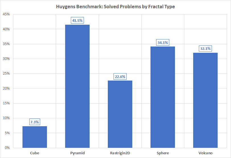
Figure 6.8: Percentage of problems solved as a function of fractal type for the Huygens test suite at

As expected from the overall results presented before, DIRECT is by far the best solver for this test suite. However, what is interesting is the bias towards the “ease” of solving fractals derived from the unit function “Pyramid” compared to the relative “hardness” of fractals derived from the unit function “Cube”. Curiously enough, DIRECT ranks relatively poorly on fractals derived from the “Cube” unit function at , easily surpassed by DE, PSWARM and BiteOpt. On all other fractals, DIRECT is largely ahead of all other optimization algorithms.