GlobOpt¶

F_opt Known	X_opt Known	Difficulty
Yes	No	Hard

The GlobOpt generator is a benchmark generator for bound-constrained global optimization test functions compared to GKLS. It is described in the paper A new class of test functions for global optimization. “GlobOpt” is not the real name of the generator, I simply used it as the original paper didn’t have a shorter acronym.

Many thanks go to Professor Marco Locatelli for providing an updated copy of the C++ source code. I have taken the original C++ code and wrapped it with Cython in order to link it to the benchmark runner.

I have compared the results of the original C++ code and the ones due to my wrapping and they are exactly the same: this is easy to see by comparing Figure 3 in the paper above with Figure 3.1 below.

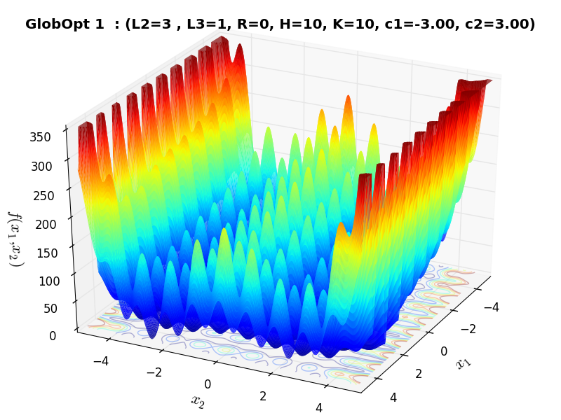
Figure 3.1: A two-dimensional GlobOpt function with $n=1$ , $L2=3$ , $L3=1$ , $K=H=10$ over the box $[−5, 5]^2$

Methodology¶

The derivation of the test functions in the GlobOpt benchmark suite is kind of complicated to describe in a short section, but I wll do my best to summarize my understanding of the original paper. The method uses functions composition to create highly multimodal, difficult to minimize test functions. The idea behind the GlobOpt generator is that local minima can be classified in “levels” - in terms of levels of difficulty. Level 1 minima ( $L_1$ ) are the easy ones to find, Level 2 minima ( $L_2$ ) are much harder and Level 3 minima ( $L_3$ ) are much, much harder. As far as I understand, the global optimum of all functions in this benchmark suite is a Level 3 minimum.

This test function generator is also very particular as the problem dimensionality is a consequence of other user-defined parameters, although the relationship between the dimensionality and those other settings is fairly straightforward and can be reverse-engineered: in this way, we can provide a desired dimensionality and adapt the other parameters to fit the generator.

As said above, there is a number of user-selectable parameters:

$n$ : the number of basic variables. Basic variables are those on which the basic multidimensional composition functions depend. $n > 1$ .

Note that they are not the unique variables of the test functions, other variables have been introduced to combine different components of the test functions (the overall number $N$ of variables on which the test functions depend can be seen in the formula below).
$L_2$ : it is the parameter which controls the number of local minimizers at Level 2.

$L_2$ is constrained to belong to the interval $\left[1, 2^{n+1}-1 \right]$ .
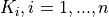
$L_3$ : the number of local minimizers at level 3. In view of the high difficulty introduced by local minimizers at Level 3, the paper sets that $L_3$ is constrained to belong to the interval $\left[1, \sqrt{n} \right]$ .
$K_i, i=1, ..., n$ : the oscillation frequencies in the one-dimensional components of the composition functions. The user has the option of fixing them all equal to a given value $K \in \left[10, 20\right]$ or to let the value of each of them be randomly chosen in the above interval.

The random choice of these values is a further source of difficulty because it introduces an anisotropic behavior of the function, i.e., a different behavior along distinct directions.
$H$ : the oscillation width: It controls the height of the barriers between neighbor local minimizers at Level 1 in the one-dimensional components of the composition functions.

$H$ is constrained to belong to the interval $\left[10, 30\right]$

Once all these settings are selected, we can actually derive the dimensionality of the problem by the following formula:

$N = n + \nu\left(L_2\right) + L_3 - 2$

Where $\nu\left(L_2\right)$ is the number of ones in the binary representation of $L_2$ . Armed with all this settings (and their constraints), we can actually reverse the formula above and generate quite a few test function by providing $L_2$ , $L_3$ and the dimensionality $N$ , then checking that the number of basic variables $n$ satisfies its constraints.

Note

The GlobOpt test suite is advertised as “Unconstrained Global Optimization Test Suite”; however, one of the main points in the paper linked above mathematically demonstrates that, even if we do not know where the exact position of the global minimum is, the algorithm guarantees that the global minimizer of the test functions lies in the interior of a sphere centered at the origin and with radius $5\sqrt{N}$ . So it was easy to assign bounds for the solvers by following this simple procedure.

The other interesting aspect of the GlobOpt generator is that, assuming we will keep the settings for $K$ and $H$ fixed and constants, then the number of “valid” test functions that can be generated is quite limited, as the constraints on the other user-settable parameters ( $n$ , $L_2$ and $L_3$ ) are stringent. This can be seen in Figure 3.2 below.

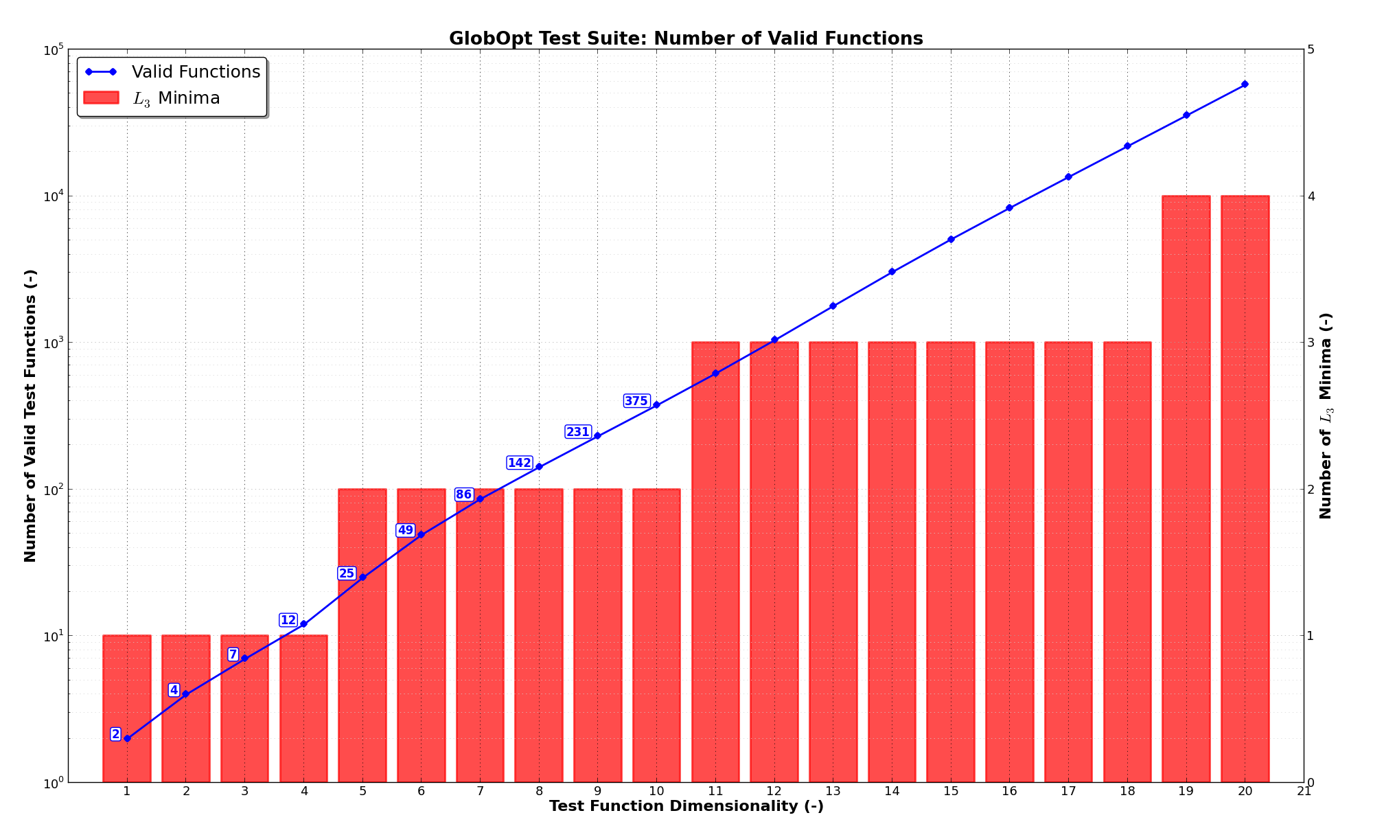
Figure 3.2: Number of “valid” test functions in the GlobOpt test suite

That said, I had no plan to keep the settings for $K$ and $H$ fixed and constants. My approach has been the following:

The dimensionality of the problem varies between $N = 2$ and $N = 5$
$L_2$ and $L_3$ are varied independently from their maximum allowable value to the minimum (thus generating very tough problems)
The parameter $K$ is either varied randomly inside the C++ code (by setting R = 0 in the Cython wrapper) or it can assume one value of either 10, 15 or 20.
$H$ can assume one value of either 10, 20 or 30.

With all these variable settings, I generated 72 valid test function per dimension, thus the current GlobOpt test suite contains 288 benchmark functions.

A few examples of 2D benchmark functions created with the GlobOpt generator can be seen in Figure 3.3.

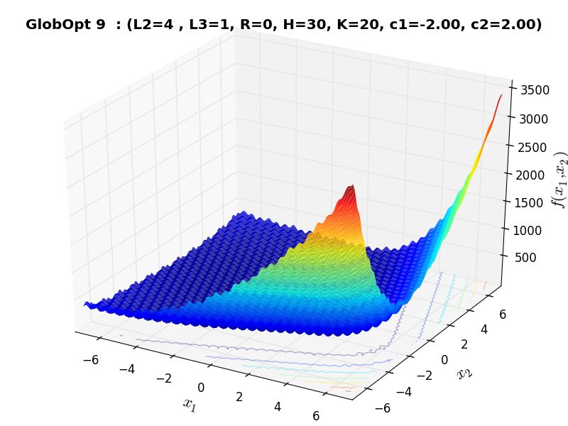
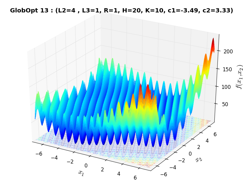
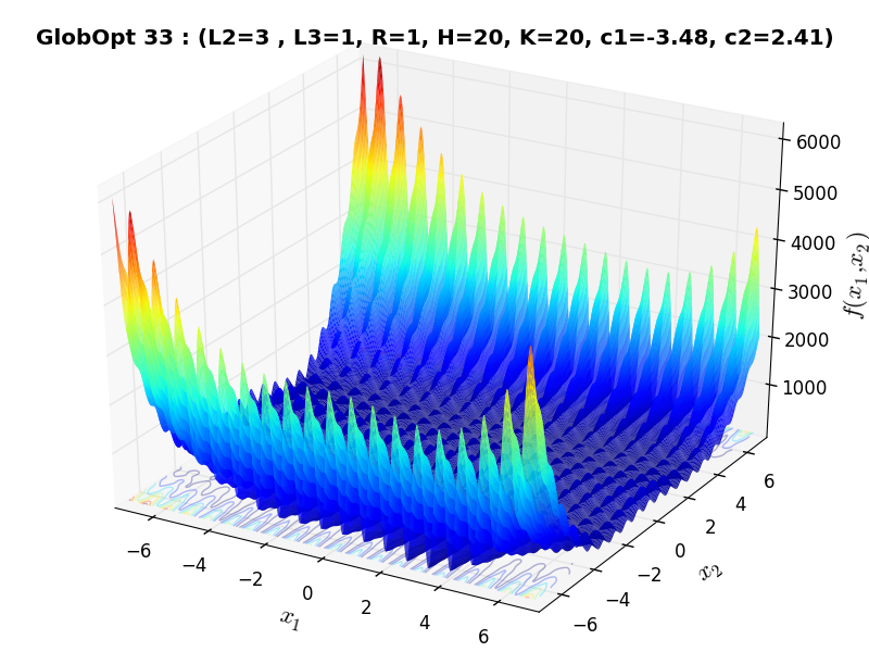
GlobOpt Function 9	GlobOpt Function 13	GlobOpt Function 33
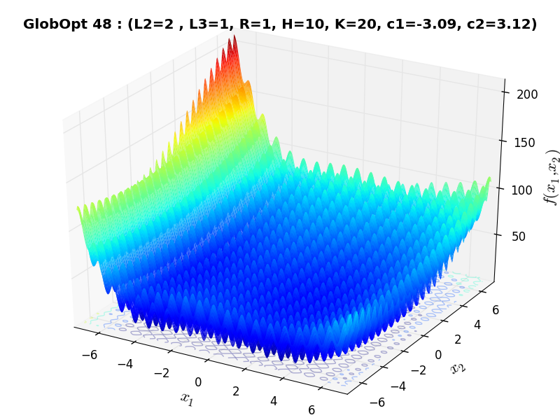
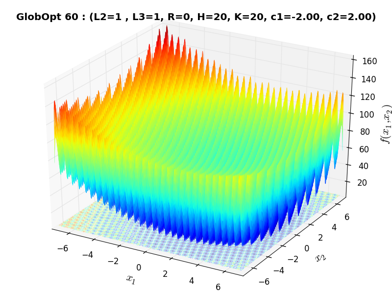
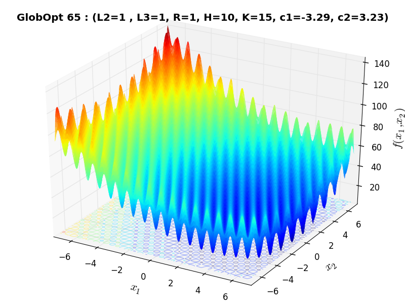
GlobOpt Function 48	GlobOpt Function 60	GlobOpt Function 65

General Solvers Performances¶

Table 3.1 below shows the overall success of all Global Optimization algorithms, considering every benchmark function, for a maximum allowable budget of $NF = 2,000$ .

Again, the GlobOpt benchmark suite is a very hard test suite, more than the GKLS one was, as the best solver (CRS2) only manages to find the global minimum in 13.9% of the cases, followed at a distance by BasinHopping and much further down by MCS and BiteOpt.

Note

The reported number of functions evaluations refers to successful optimizations only.

**Table 3.1**: Solvers performances on the GlobOpt benchmark suite at NF = 2,000
Optimization Method	Overall Success (%)	Functions Evaluations
AMPGO	1.39%	1,232
BasinHopping	10.42%	1,097
BiteOpt	6.25%	1,020
CMA-ES	0.35%	1,167
CRS2	13.89%	1,201
DE	4.51%	1,677
DIRECT	3.82%	1,306
DualAnnealing	5.56%	864
LeapFrog	1.39%	268
MCS	6.94%	1,170
PSWARM	0.00%	0
SCE	0.35%	1,598
SHGO	0.69%	47

These results are also depicted in Figure 3.4, which shows that CRS2 is the better-performing optimization algorithm, followed by BasinHopping and MCS.

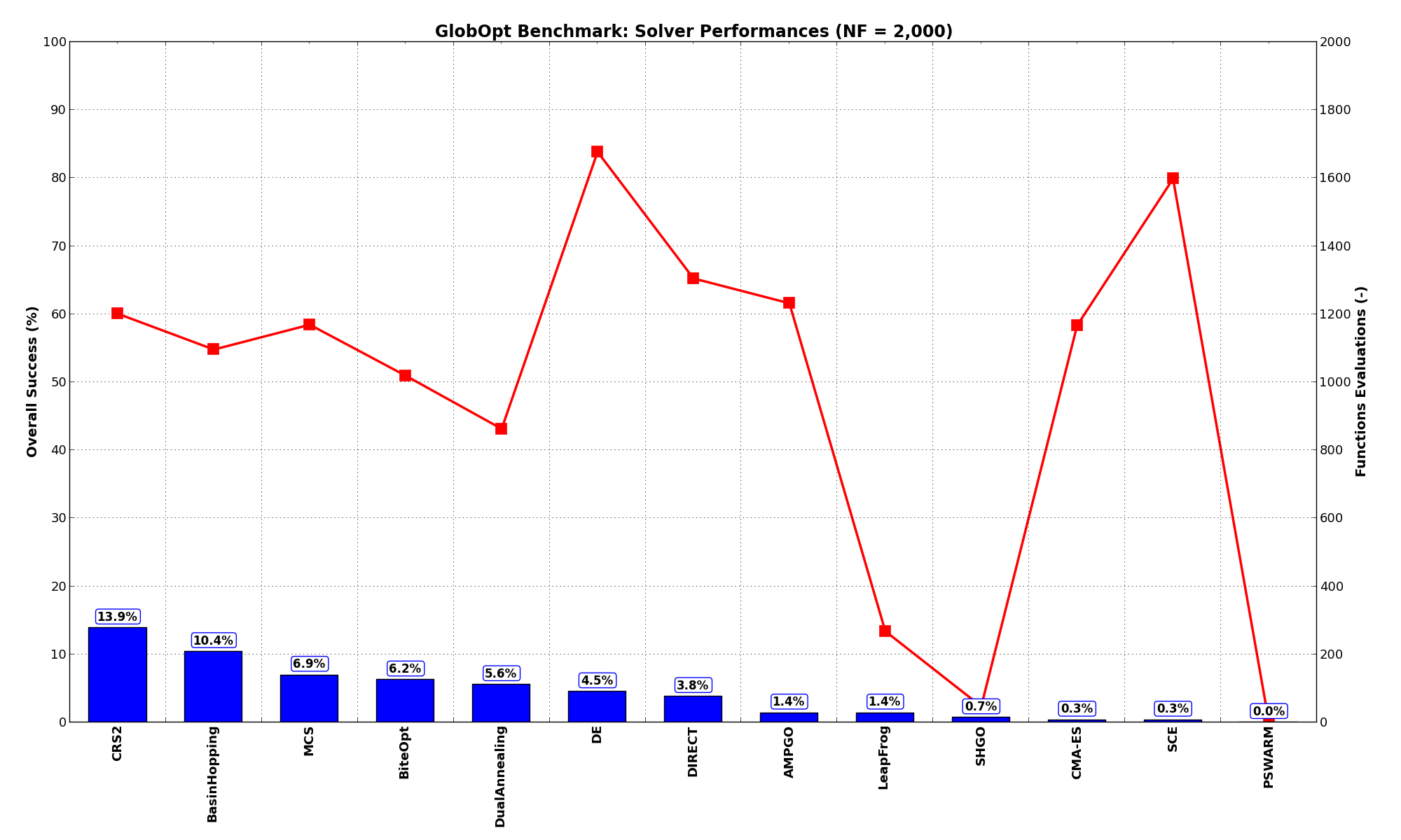
Optimization algorithms performances on the GlobOpt test suite at :math:`NF = 2,000`

Figure 3.4: Optimization algorithms performances on the GlobOpt test suite at $NF = 2,000$

Pushing the available budget to a very generous $NF = 10,000$ , the results show MCS taking the lead on other solvers (about 3% more problems solved compared to the second best, BasinHopping). The results are also shown visually in Figure 3.5.

**Table 3.2**: Solvers performances on the GlobOpt benchmark suite at NF = 10,000
Optimization Method	Overall Success (%)	Functions Evaluations
AMPGO	5.90%	3,955
BasinHopping	20.83%	2,250
BiteOpt	10.76%	2,624
CMA-ES	3.12%	6,164
CRS2	18.40%	2,366
DE	10.76%	4,427
DIRECT	10.42%	3,529
DualAnnealing	7.29%	1,340
LeapFrog	1.39%	268
MCS	23.96%	3,754
PSWARM	7.29%	3,585
SCE	3.82%	5,893
SHGO	3.82%	5,289

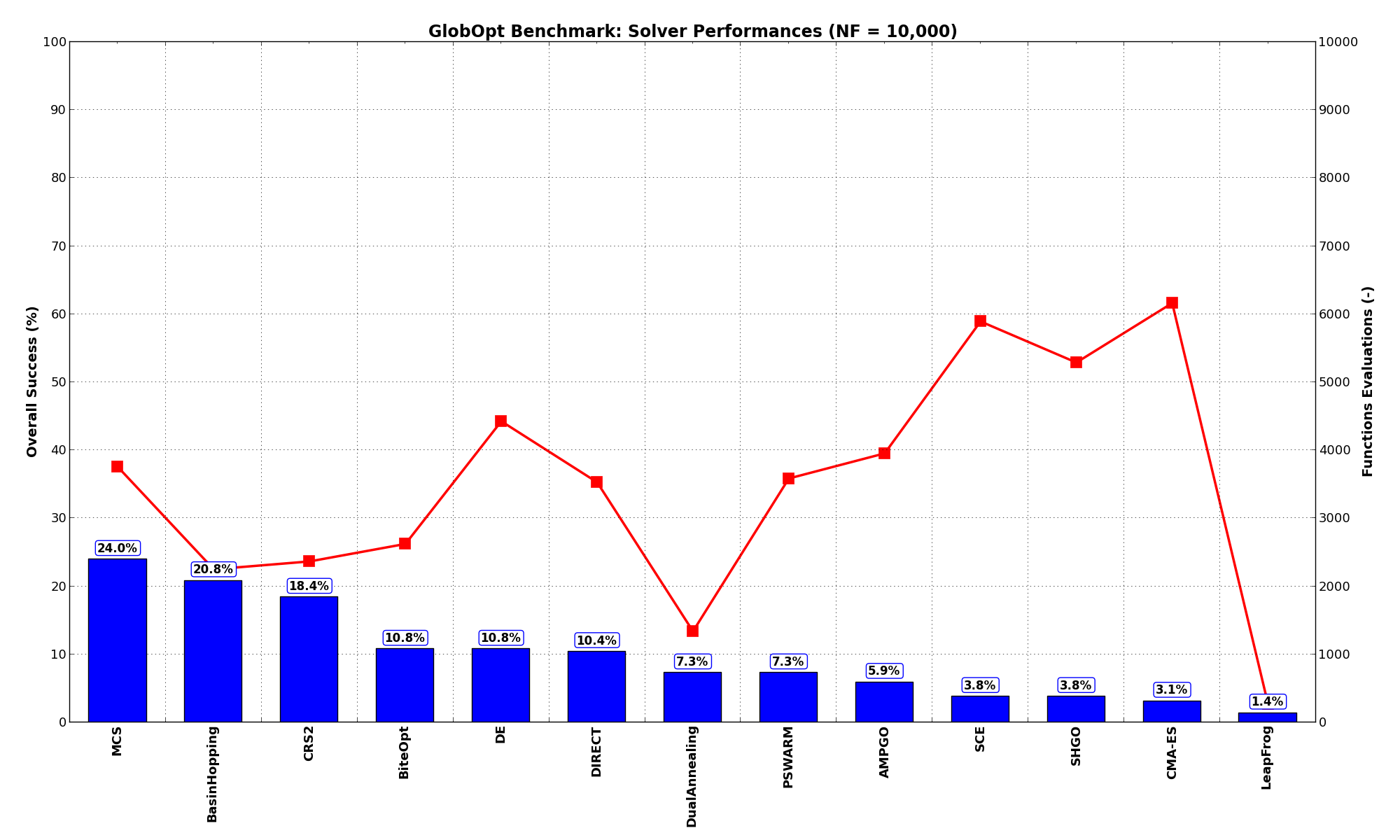
Optimization algorithms performances on the GlobOpt test suite at :math:`NF = 10,000`

Figure 3.5: Optimization algorithms performances on the GlobOpt test suite at $NF = 10,000$

Since I was super annoyed that none of the Global Optimization algorithms were doing any better than 24% solved problems even with a very generous budget of function evaluations of $NF = 10,000$ , for this test suite only I decided to push the limits even more and allow an extended $NF = 20,000$ and $NF = 50,000$ budget limit, just to see if any difference could be spotted - or any change in the algorithm performances.

Alas, as Figure 3.6 shows, even the best solver ( MCS) cannot get better than 36.5% of the problems solved. What is interesting, though, is the much improved performances of one of the SciPy solvers, SHGO, which moves from 4% to 29% of all global minimum found.

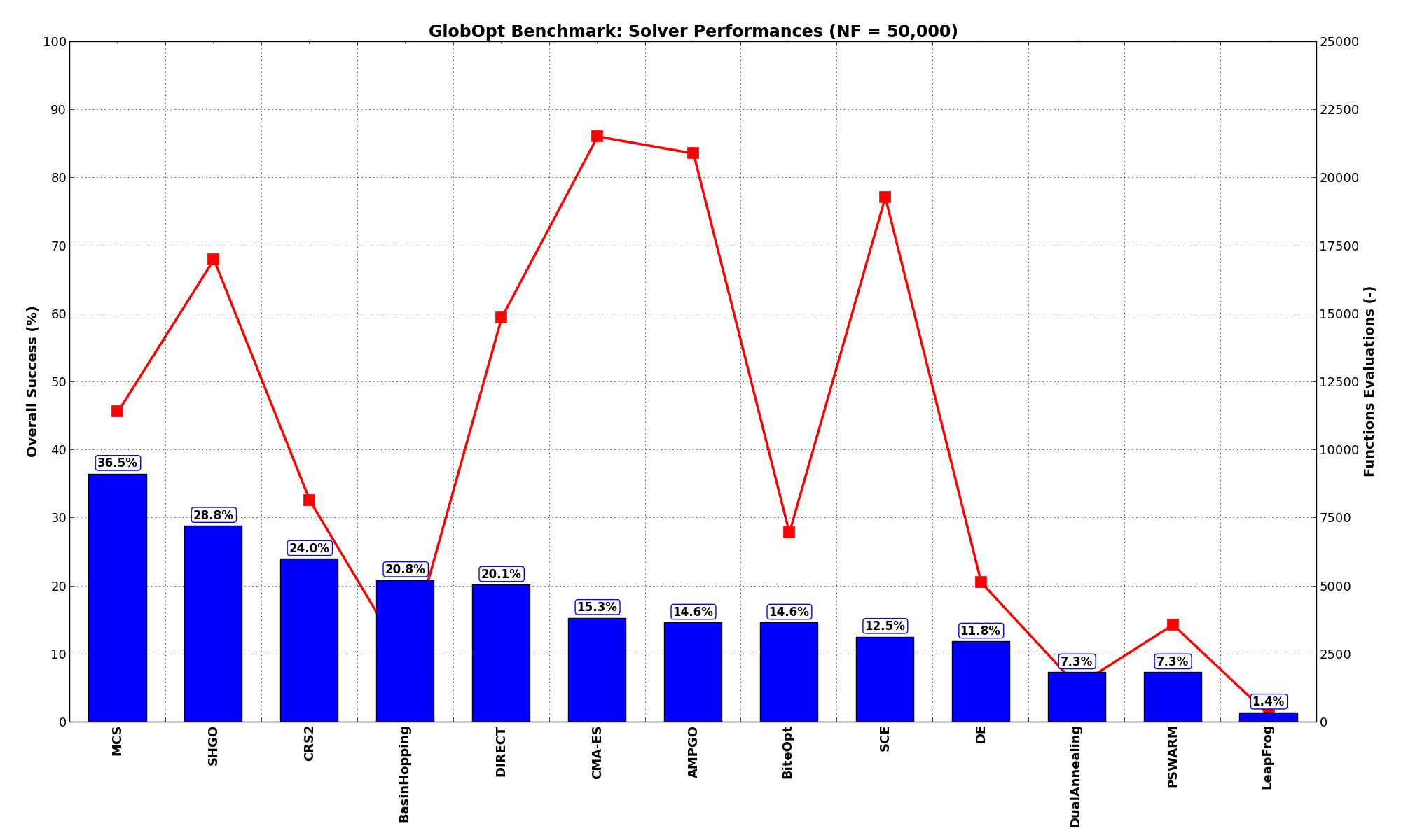
Optimization algorithms performances on the GlobOpt test suite at :math:`NF = 50,000`

Figure 3.6: Optimization algorithms performances on the GlobOpt test suite at $NF = 50,000$

Sensitivities on Functions Evaluations Budget¶

It is also interesting to analyze the success of an optimization algorithm based on the fraction (or percentage) of problems solved given a fixed number of allowed function evaluations, let’s say 100, 200, 300,... 2000, 5000, 10000.

In order to do that, we can present the results using two different types of visualizations. The first one is some sort of “small multiples” in which each solver gets an individual subplot showing the improvement in the number of solved problems as a function of the available number of function evaluations - on top of a background set of grey, semi-transparent lines showing all the other solvers performances.

This visual gives an indication of how good/bad is a solver compared to all the others as function of the budget available. Results are shown in Figure 3.7.

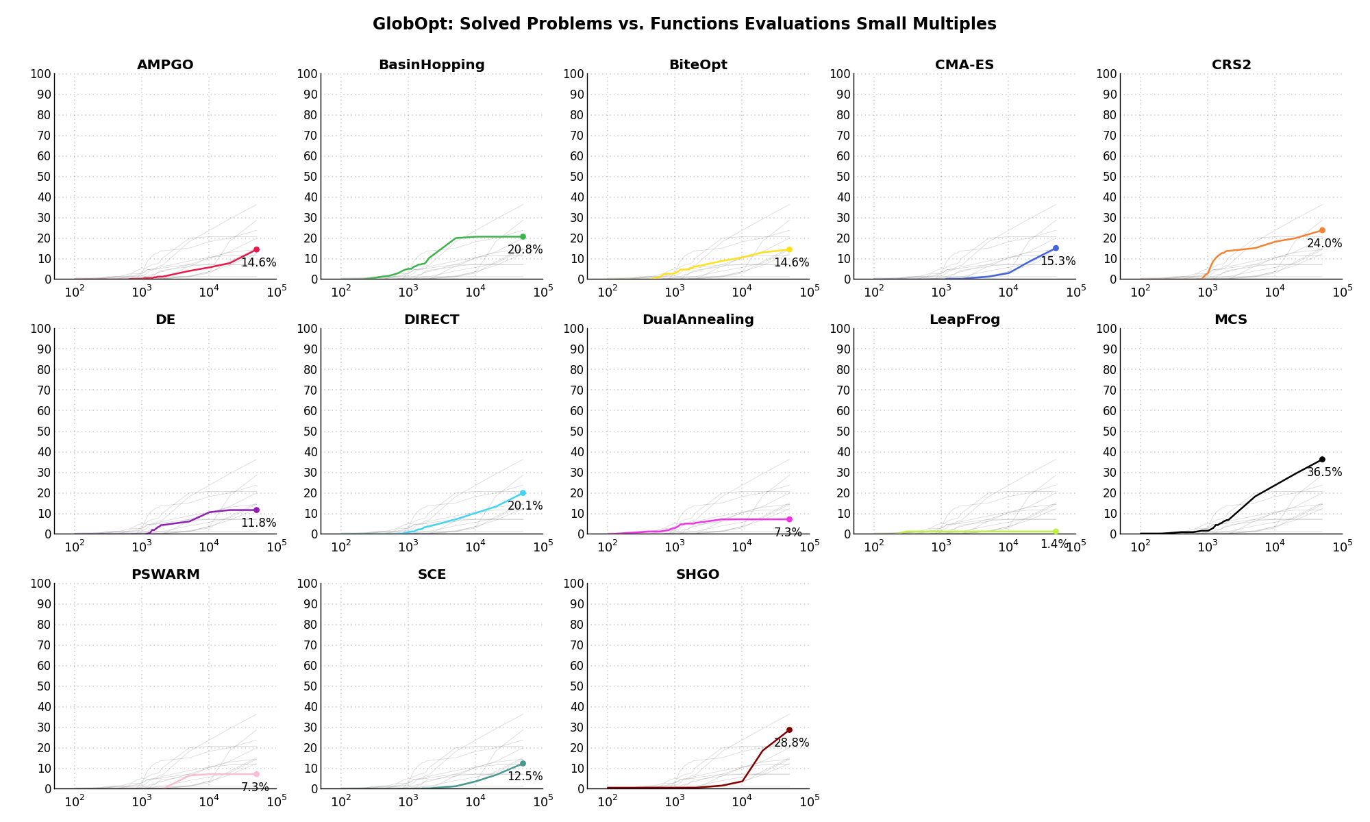
Figure 3.7: Percentage of problems solved given a fixed number of function evaluations on the GlobOpt test suite

The second type of visualization is sometimes referred as “Slopegraph” and there are many variants on the plot layout and appearance that we can implement. The version shown in Figure 3.8 aggregates all the solvers together, so it is easier to spot when a solver overtakes another or the overall performance of an algorithm while the available budget of function evaluations changes.

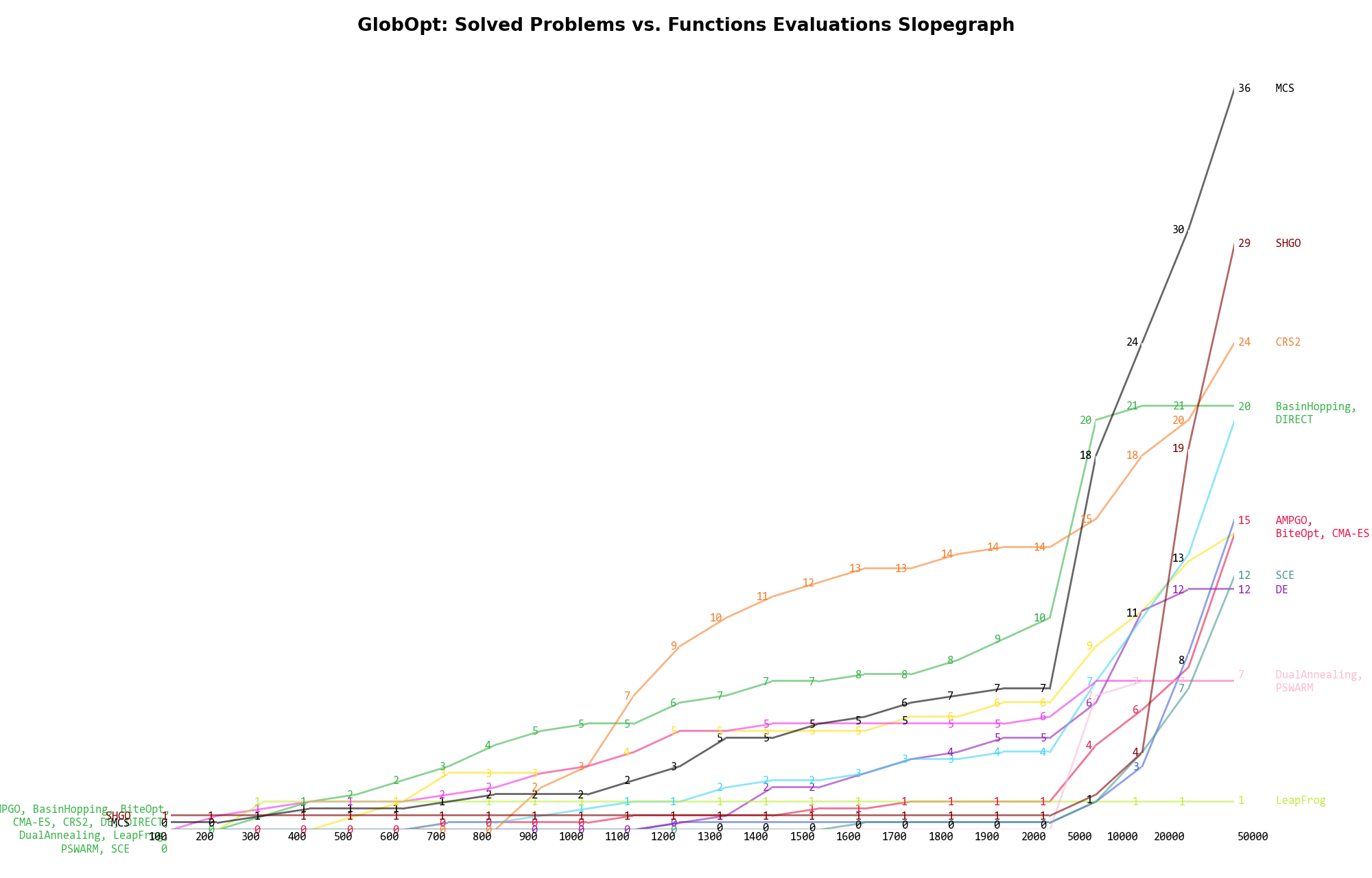
Figure 3.8: Percentage of problems solved given a fixed number of function evaluations on the GlobOpt test suite

A few obvious conclusions we can draw from these pictures are:

For this specific benchmark test suite, if you have a very limited budget in terms of function evaluations, then none of the solvers is going to get you any good result whatsoever. The best performing algorithms below $NF = 2,000$ are CRS2 and BasinHopping, with meagre 14% and 10% solved problems respectively.
There is a distinct improvements of performances for solvers like MCS and SHGO when the maximum number of function evaluations is relaxed (to very high limits though).

Dimensionality Effects¶

Since I used the GlobOpt test suite to generate test functions with dimensionality ranging from 2 to 5, it is interesting to take a look at the solvers performances as a function of the problem dimensionality. Of course, in general it is to be expected that for larger dimensions less problems are going to be solved - although it is not always necessarily so as it also depends on the function being generated. Results are shown in Table 3.3 .

**Table 3.3**: Dimensionality effects on the GlobOpt benchmark suite at NF = 2,000
Solver	N = 2	N = 3	Overall
AMPGO	1.4	4.2	1.4
BasinHopping	40.3	1.4	10.4
BiteOpt	25.0	0.0	6.2
CMA-ES	1.4	0.0	0.3
CRS2	52.8	2.8	13.9
DE	18.1	0.0	4.5
DIRECT	15.3	0.0	3.8
DualAnnealing	22.2	0.0	5.6
LeapFrog	5.6	0.0	1.4
MCS	26.4	1.4	6.9
PSWARM	0.0	0.0	0.0
SCE	1.4	0.0	0.3
SHGO	2.8	0.0	0.7

Figure 3.9 shows the same results in a visual way.

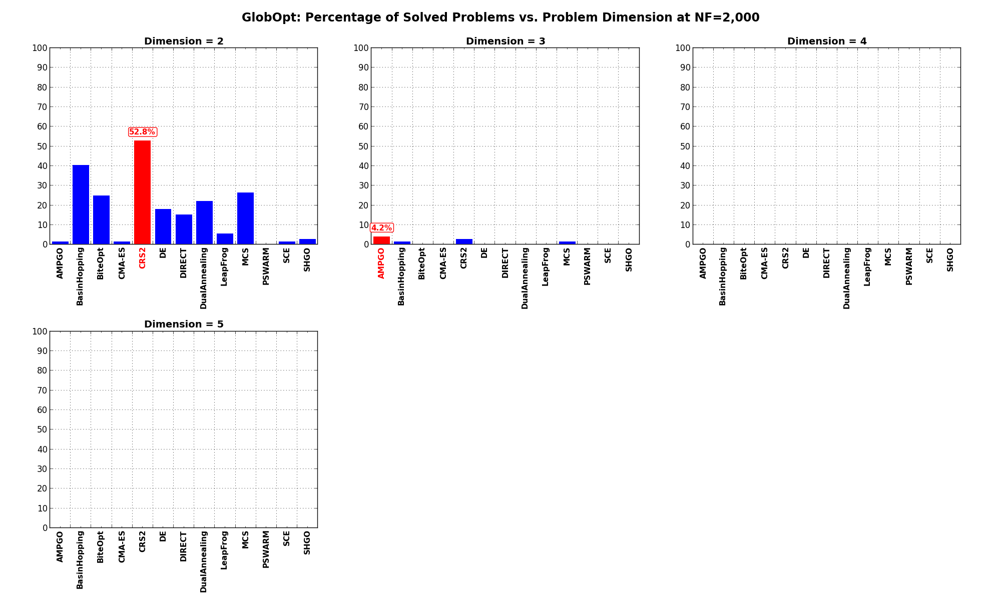
Percentage of problems solved as a function of problem dimension at :math:`NF = 2,000`

Figure 3.9: Percentage of problems solved as a function of problem dimension for the GlobOpt test suite at $NF = 2,000$

What we can infer from the table and the figure is that, for lower dimensionality problems ( $NF < 3$ ), the CRS2 algorithm has a significant advantage over all other algorithms, although the SciPy optimizer BasinHopping is not too far behind. For higher dimensionality problems ( $N \geq 3$ ), the performance degradations are noticeable for all solvers, and none of the solvers is able to show any meaningful and strong result.

Pushing the available budget to a very generous $NF = 10,000$ , the results show MCS taking a significant lead on other solvers, but only on very low dimensionality problems with $N = 2$ . For higher dimensionality problems a solver like CRS2 or DE is a much safe option, although the performances are not spectacular at all.

The results for the benchmarks at $NF = 10,000$ are displayed in Table 3.4 and Figure 3.10.

**Table 3.4**: Dimensionality effects on the GlobOpt benchmark suite at NF = 10,000
Solver	N = 2	N = 3	N = 4	N = 5	Overall
AMPGO	18.1	5.6	0.0	0.0	5.9
BasinHopping	65.3	11.1	5.6	1.4	20.8
BiteOpt	37.5	4.2	0.0	1.4	10.8
CMA-ES	12.5	0.0	0.0	0.0	3.1
CRS2	52.8	12.5	8.3	0.0	18.4
DE	20.8	12.5	8.3	1.4	10.8
DIRECT	34.7	6.9	0.0	0.0	10.4
DualAnnealing	29.2	0.0	0.0	0.0	7.3
LeapFrog	5.6	0.0	0.0	0.0	1.4
MCS	84.7	11.1	0.0	0.0	24.0
PSWARM	26.4	2.8	0.0	0.0	7.3
SCE	15.3	0.0	0.0	0.0	3.8
SHGO	15.3	0.0	0.0	0.0	3.8

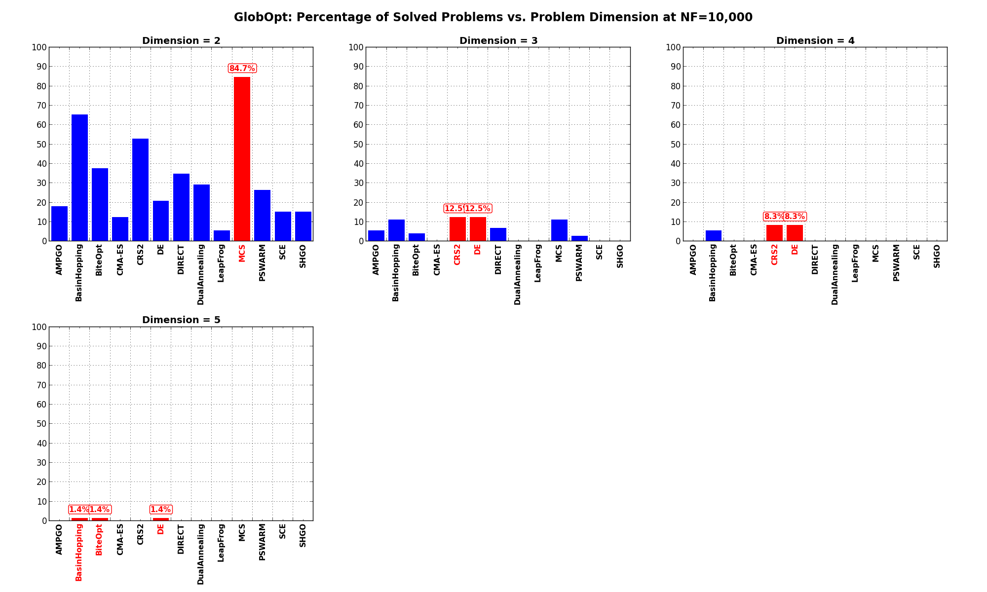
Percentage of problems solved as a function of problem dimension at :math:`NF = 10,000`

Figure 3.10: Percentage of problems solved as a function of problem dimension for the GlobOpt test suite at $NF = 10,000$

GlobOpt¶

Methodology¶

General Solvers Performances¶

Sensitivities on Functions Evaluations Budget¶

Dimensionality Effects¶

Table Of Contents

Previous topic

Next topic

This Page

Navigation

GlobOpt¶

Methodology¶

General Solvers Performances¶

Sensitivities on Functions Evaluations Budget¶

Dimensionality Effects¶

Table Of Contents

Previous topic

Next topic

This Page

Quick search

Navigation