GKLS¶

F_opt Known	X_opt Known	Difficulty
Yes	Yes	Hard

The GKLS generator is a very popular benchmark generator for bound-constrained global optimization test functions. It is described in the paper Software for Generation of Classes of Test Functions with Known Local and Global Minima for Global Optimization. I have taken the original C code (available at http://netlib.org/toms/) and converted it to Python.

The conversion was not strictly necessary but I didn’t feel confident enough to modify the C code and wrap it with Cython in order to allow a two way communication between GKLS and the benchmark runner. In any case, I have compared the results of the original C code and of my translation ad they are exactly the same: this is easy to see by comparing Figure 1 in the paper above with Figure 2.1 below.

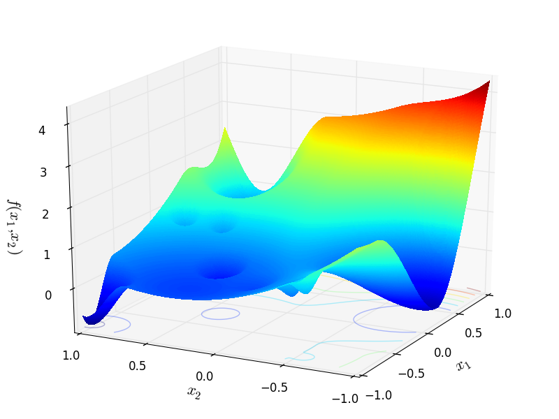
Figure 2.1: GKLS function number 9 from a class of two-dimensional D-type test functions with 10 local minima

Methodology¶

The GKLS generator is a procedure for generating three types (non-differentiable, continuously differentiable, and twice continuously differentiable) of classes of test functions with known local and global minima for multiextremal multidimensional box-constrained global optimization.

The procedure consists of defining a convex quadratic function systematically distorted by polynomials in order to introduce local minima. Each test class provided by the GKLS generator consists of 100 functions constructed randomly and is defined by the following parameters:

Problem dimension
Number of local minima
Value of the global minimum
Radius of the attraction region of the global minimizer
Distance from the global minimizer to the vertex of the quadratic function

Since the user is given freedom in the choice of dimension, number of local minima, radius of the attraction region of the global minimizer and distance from the global minimizer to the vertex of the quadratic function, my approach in generating the test functions has been the following:

The problem dimension $N$ ranges from 2 to 6
For each dimension, there are three types of functions generated by GKLS: non-differentiable (ND), continuously differentiable (D1) and twice continuously differentiable (D2)
For each dimension, GKLS generates 100 functions

In that way, we have 5 possible dimensions, 3 possible function types and 100 different functions per function types. This gives a set of 1,500 test functions. In order to give some variability, I also decided to play with the other free parameters of the generator, and namely:

The number of local minima is chosen randomly between 3 and 100 for each function
The distance from the global minimizer to the vertex of the quadratic function is chosen randomly between a very small number ( $10^{-15}$ ) and half of the domain bounds (which is $-1 \leq x \leq 1$ )
The radius of the attraction region of the global minimizer is chosen randomly between a very small number ( $10^{-15}$ ) and half of the distance from the global minimizer to the vertex of the quadratic function (defined above)

As an example of the differences between ND, D1 and D2 functions, Figure 2.2 below contains some 3D representations of some of the benchmark functions in the GKLS test suite.

Note

For all test problems in the GKLS test suite, and for all dimensions, I have arbitrarily set the value of the global minimum at $f_{opt} = 0.5$ . The default in the original C code is $f_{opt} = -1.0$ but it’s relatively easy to change by manipulating the two “global” variables GKLS_GLOBAL_MIN_VALUE and GKLS_PARABOLOID_MIN, as the test suite requires $\textrm{GKLS\_PARABOLOID\_MIN} > \textrm{GKLS\_GLOBAL\_MIN\_VALUE}$ .

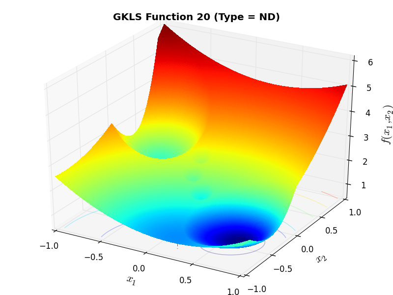
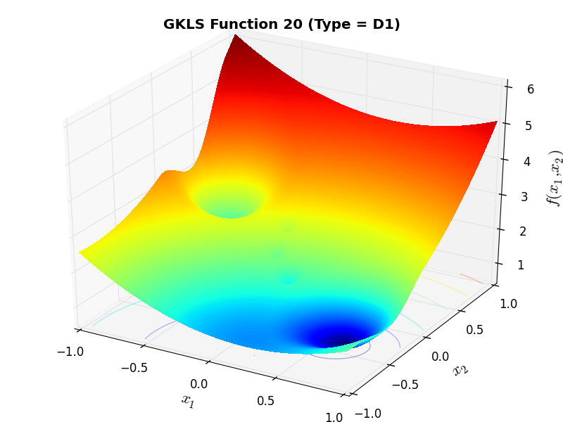
GKLS Function 20 (ND)	GKLS Function 20 (D1)	GKLS Function 20 (D2)
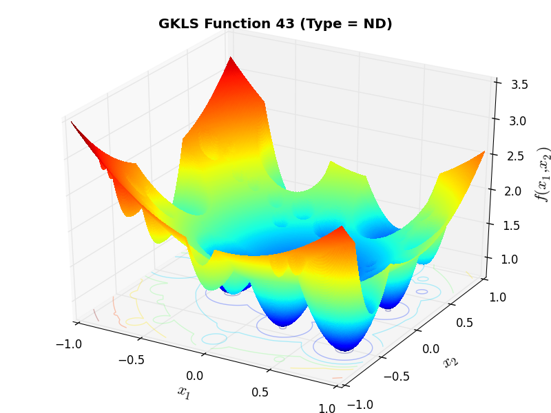
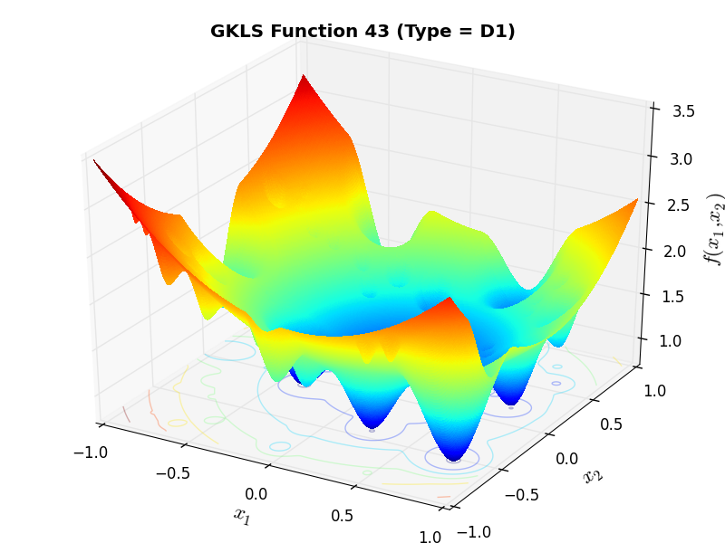
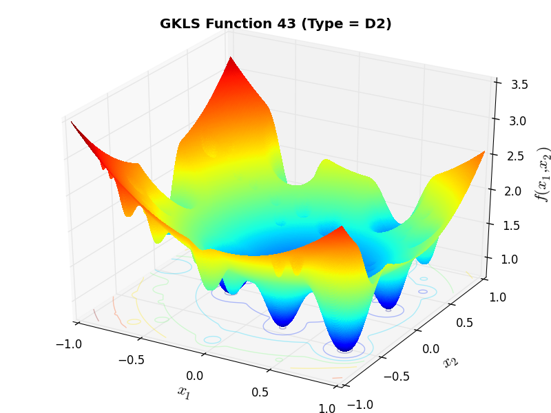
GKLS Function 43 (ND)	GKLS Function 43 (D1)	GKLS Function 43 (D2)

General Solvers Performances¶

Table 2.1 below shows the overall success of all Global Optimization algorithms, considering every benchmark function, for a maximum allowable budget of $NF = 2,000$ .

It is clear at first sight that the GKLS benchmark suite is a much tougher cookie than the SciPy Extended one, as the best solver ( MCS) only manages to find the global minimum in 28.5% of the cases, while the best SciPy optimization routines are trailing slightly behind at 24% for DualAnnealing and 23.3% for SHGO.

Among the solvers that pass the 20% threshold of solved problems, we can see that DIRECT is the “cheapest” one, using 446 functions evaluations on average, followed by DualAnnealing, MCS and SHGO.

Note

The reported number of functions evaluations refers to successful optimizations only.

**Table 2.1**: Solvers performances on the GKLS benchmark suite at NF = 2,000
Optimization Method	Overall Success (%)	Functions Evaluations
AMPGO	14.13%	651
BasinHopping	15.53%	721
BiteOpt	18.60%	628
CMA-ES	7.07%	745
CRS2	12.07%	826
DE	13.73%	1,036
DIRECT	21.33%	446
DualAnnealing	24.00%	529
LeapFrog	7.53%	227
MCS	28.53%	610
PSWARM	9.93%	1,664
SCE	12.07%	604
SHGO	23.27%	639

These results are also depicted in Figure 2.3, which shows that MCS is the better-performing optimization algorithm, closely followed by DualAnnealing and SHGO.

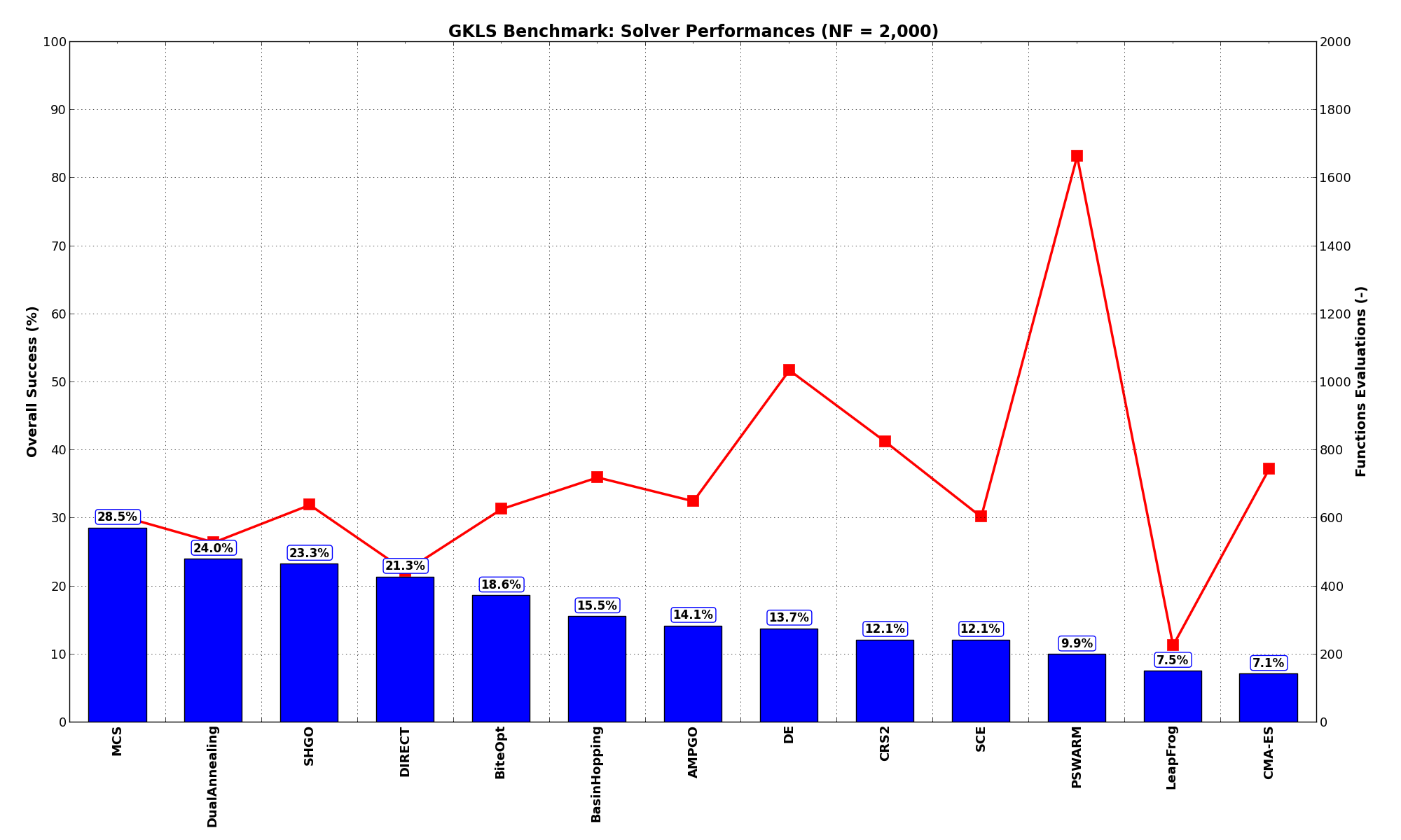
Optimization algorithms performances on the GKLS test suite at :math:`NF = 2,000`

Figure 2.3: Optimization algorithms performances on the GKLS test suite at $NF = 2,000$

Pushing the available budget to a very generous 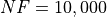$NF = 10,000$ , the results show MCS taking a larger lead on other solvers (about 9% more problems solved compared to the second best, DualAnnealing) and AMPGO gaining quite some ground compared to the lower budget $NF = 2,000$ . There is also a significant uptick in performances for PSWARM as shown in Table 2.2 and Figure 2.4.

**Table 2.2**: Solvers performances on the GKLS benchmark suite at NF = 10,000
Optimization Method	Overall Success (%)	Functions Evaluations
AMPGO	26.60%	2,734
BasinHopping	19.40%	1,378
BiteOpt	22.80%	1,422
CMA-ES	12.47%	2,480
CRS2	13.73%	1,057
DE	19.40%	1,948
DIRECT	28.60%	1,478
DualAnnealing	30.07%	1,257
LeapFrog	7.53%	227
MCS	39.27%	1,658
PSWARM	19.47%	2,036
SCE	13.80%	1,123
SHGO	29.53%	1,808

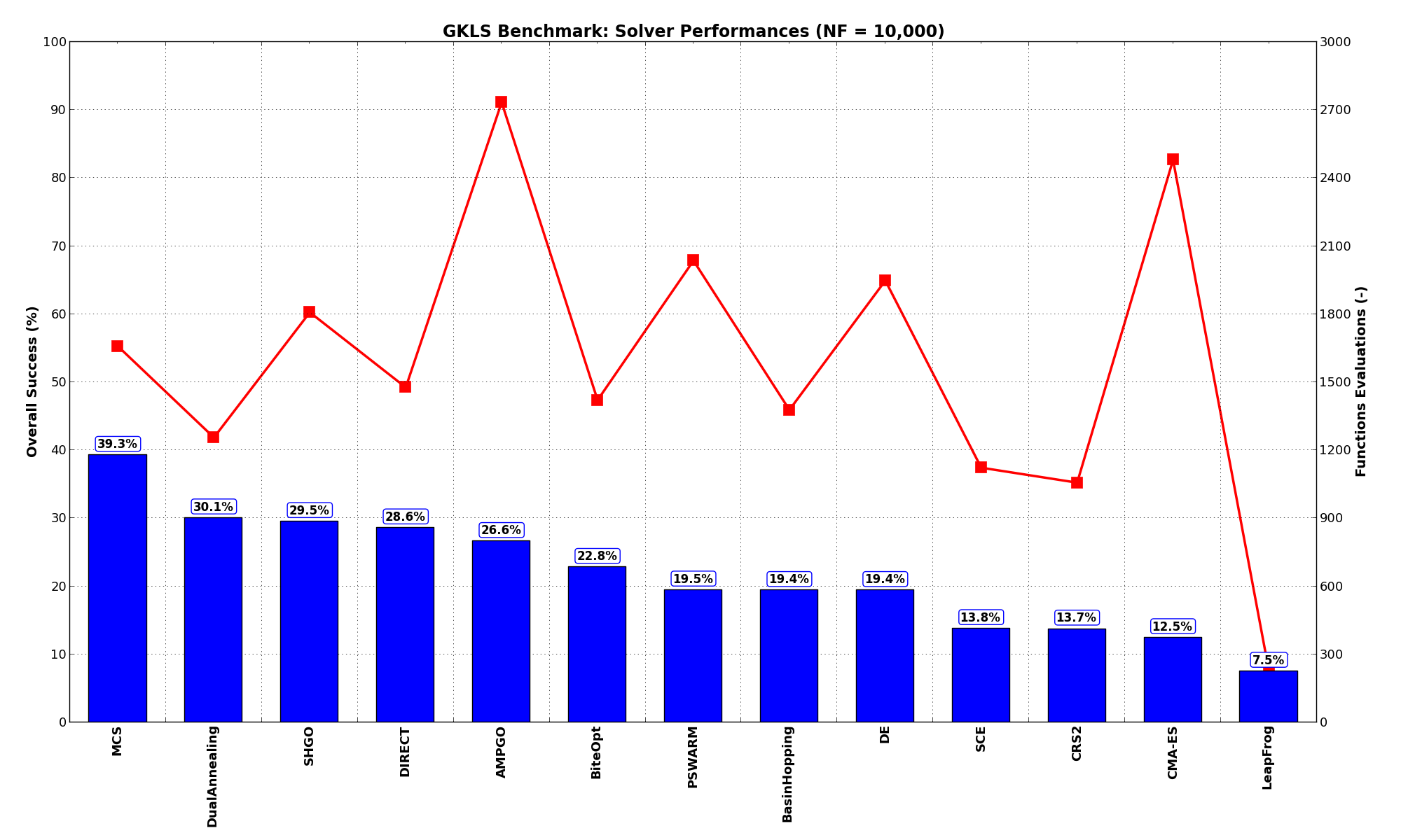
Optimization algorithms performances on the GKLS test suite at :math:`NF = 10,000`

Figure 2.4: Optimization algorithms performances on the GKLS test suite at $NF = 10,000$

Sensitivities on Functions Evaluations Budget¶

It is also interesting to analyze the success of an optimization algorithm based on the fraction (or percentage) of problems solved given a fixed number of allowed function evaluations, let’s say 100, 200, 300,... 2000, 5000, 10000.

In order to do that, we can present the results using two different types of visualizations. The first one is some sort of “small multiples” in which each solver gets an individual subplot showing the improvement in the number of solved problems as a function of the available number of function evaluations - on top of a background set of grey, semi-transparent lines showing all the other solvers performances.

This visual gives an indication of how good/bad is a solver compared to all the others as function of the budget available. Results are shown in Figure 2.5.

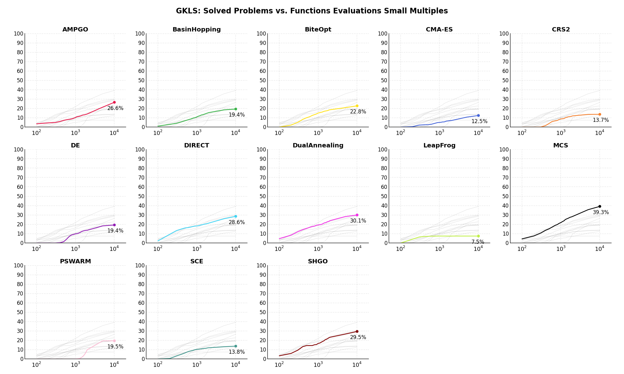
Figure 2.5: Percentage of problems solved given a fixed number of function evaluations on the GKLS test suite

The second type of visualization is sometimes referred as “Slopegraph” and there are many variants on the plot layout and appearance that we can implement. The version shown in Figure 2.6 aggregates all the solvers together, so it is easier to spot when a solver overtakes another or the overall performance of an algorithm while the available budget of function evaluations changes.

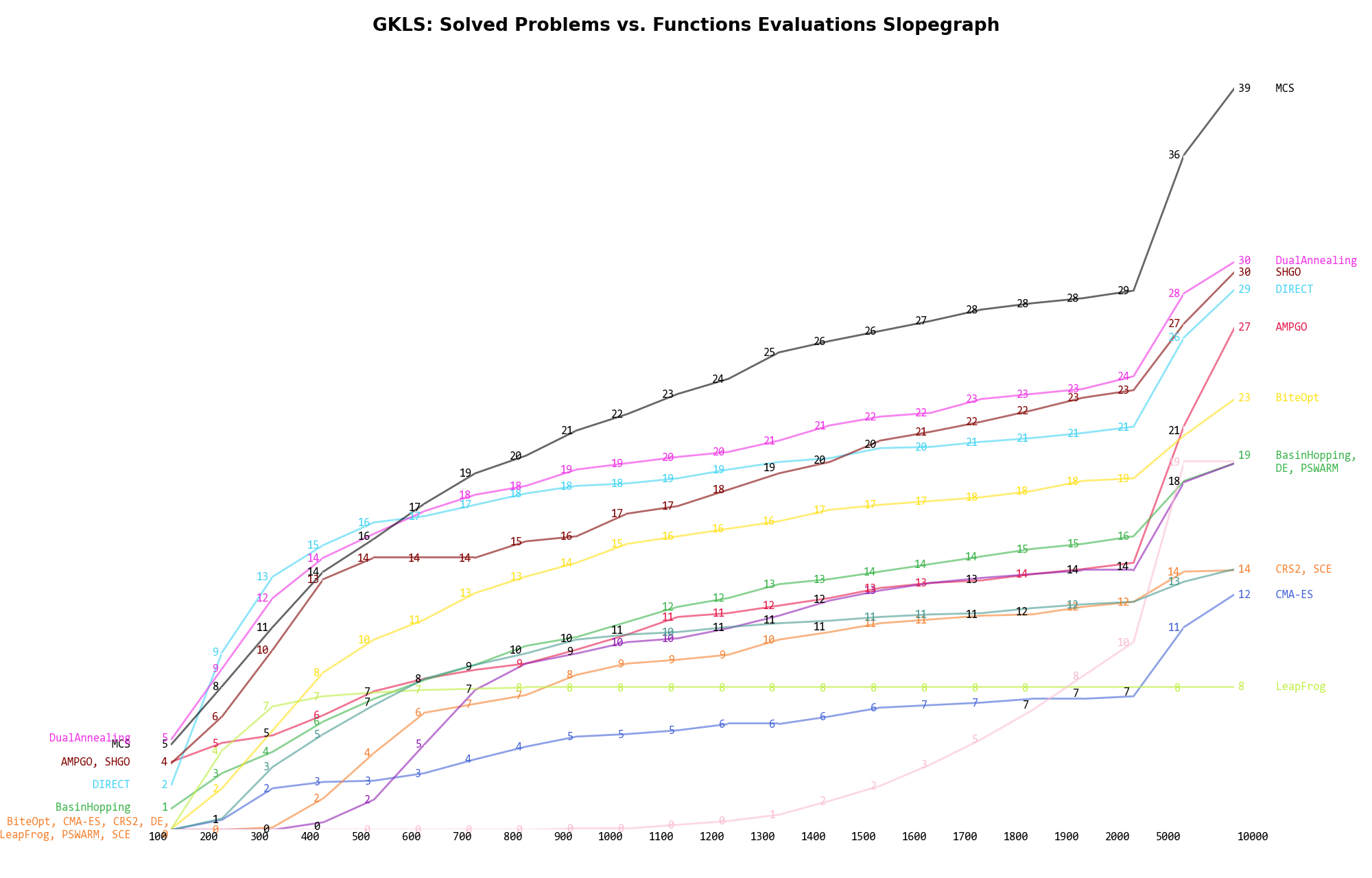
Figure 2.6: Percentage of problems solved given a fixed number of function evaluations on the GKLS test suite

A few obvious conclusions we can draw from these pictures are:

For this specific benchmark test suite, if you have a very limited budget in terms of function evaluations, then MCS, SHGO, DualAnnealing and DIRECT are a very good choice: they solve around 15% of all problems in 500 function evaluations or less.
There is a distinct separation of performances between MCS and the other solvers as soon as the number of functions evaluations raises above $NF = 1,000$ .
Pretty much all algorithms benefit from a larger budget (i.e., $NF = 10,000$ ) - obviously - but the improvement is much more evident for solvers like MCS (+10%), AMPGO (+13%) and PSWARM (+9%) compared to a budget of $NF = 2,000$ .

Dimensionality Effects¶

Since I used the GKLS test suite to generate test functions with dimensionality ranging from 2 to 6, it is interesting to take a look at the solvers performances as a function of the problem dimensionality. Of course, in general it is to be expected that for larger dimensions less problems are going to be solved - although it is not always necessarily so as it also depends on the function being generated. Results are shown in Table 2.3 .

**Table 2.3**: Dimensionality effects on the GKLS benchmark suite at NF = 2,000
Solver	N = 2	N = 3	N = 4	N = 5	N = 6	Overall
AMPGO	43.7	16.3	4.7	4.3	1.7	14.1
BasinHopping	50.3	18.7	8.3	0.0	0.3	15.5
BiteOpt	46.7	16.3	14.3	8.7	7.0	18.6
CMA-ES	27.3	5.3	2.3	0.3	0.0	7.1
CRS2	35.3	15.3	7.3	2.3	0.0	12.1
DE	49.0	18.7	1.0	0.0	0.0	13.7
DIRECT	65.7	28.3	10.3	2.0	0.3	21.3
DualAnnealing	68.3	25.0	13.7	8.3	4.7	24.0
LeapFrog	25.7	7.7	1.7	1.7	1.0	7.5
MCS	75.0	42.3	15.3	5.0	5.0	28.5
PSWARM	44.0	4.7	1.0	0.0	0.0	9.9
SCE	45.0	10.7	4.3	0.0	0.3	12.1
SHGO	72.3	32.7	10.3	1.0	0.0	23.3

Figure 2.7 shows the same results in a visual way.

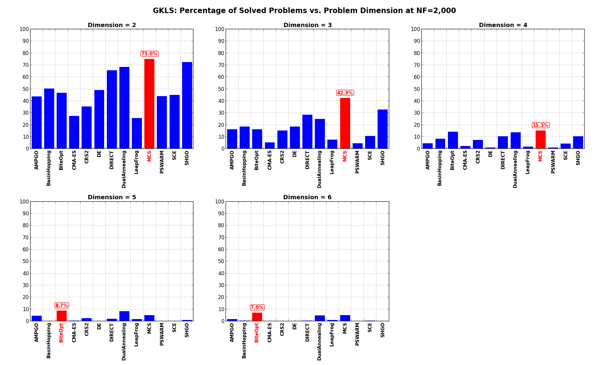
Percentage of problems solved as a function of problem dimension at :math:`NF = 2,000`

Figure 2.7: Percentage of problems solved as a function of problem dimension for the GKLS test suite at $NF = 2,000$

What we can infer from the table and the figure is that, for lower dimensionality problems ( $NF \leq 3$ ), the MCS algorithm has some advantage over other solvers, although the SciPy optimizers SHGO and DualAnnealing are not very far behind. For higher dimensionality problems ( $N \geq 5$ ), the performance degradations are noticeable for all solvers, and a new winner shows up: BiteOpt, closely followed by MCS and DualAnnealing.

Pushing the available budget to a very generous $NF = 10,000$ , the results show MCS taking a larger lead on other solvers, especially on problems with $N = 3`and :math:`N = 4$ . For higher dimensionality problems ( $N \geq 5$ ) DualAnnealing starts shining more than any other optimizer.

The results for the benchmarks at $NF = 10,000$ are displayed in Table 2.4 and Figure 2.8.

**Table 2.4**: Dimensionality effects on the GKLS benchmark suite at NF = 10,000
Solver	N = 2	N = 3	N = 4	N = 5	N = 6	Overall
AMPGO	67.3	34.3	16.7	8.3	6.3	26.6
BasinHopping	57.0	25.7	10.7	2.0	1.7	19.4
BiteOpt	62.0	18.7	16.0	9.7	7.7	22.8
CMA-ES	41.7	12.3	6.0	2.0	0.3	12.5
CRS2	35.7	17.3	7.7	4.7	3.3	13.7
DE	49.3	20.0	11.7	11.3	4.7	19.4
DIRECT	79.0	35.7	19.3	8.0	1.0	28.6
DualAnnealing	72.0	33.3	19.0	14.3	11.7	30.1
LeapFrog	25.7	7.7	1.7	1.7	1.0	7.5
MCS	88.7	59.0	33.3	9.3	6.0	39.3
PSWARM	62.7	20.0	11.3	3.3	0.0	19.5
SCE	48.7	12.7	5.7	0.7	1.3	13.8
SHGO	84.3	47.7	10.3	5.3	0.0	29.5

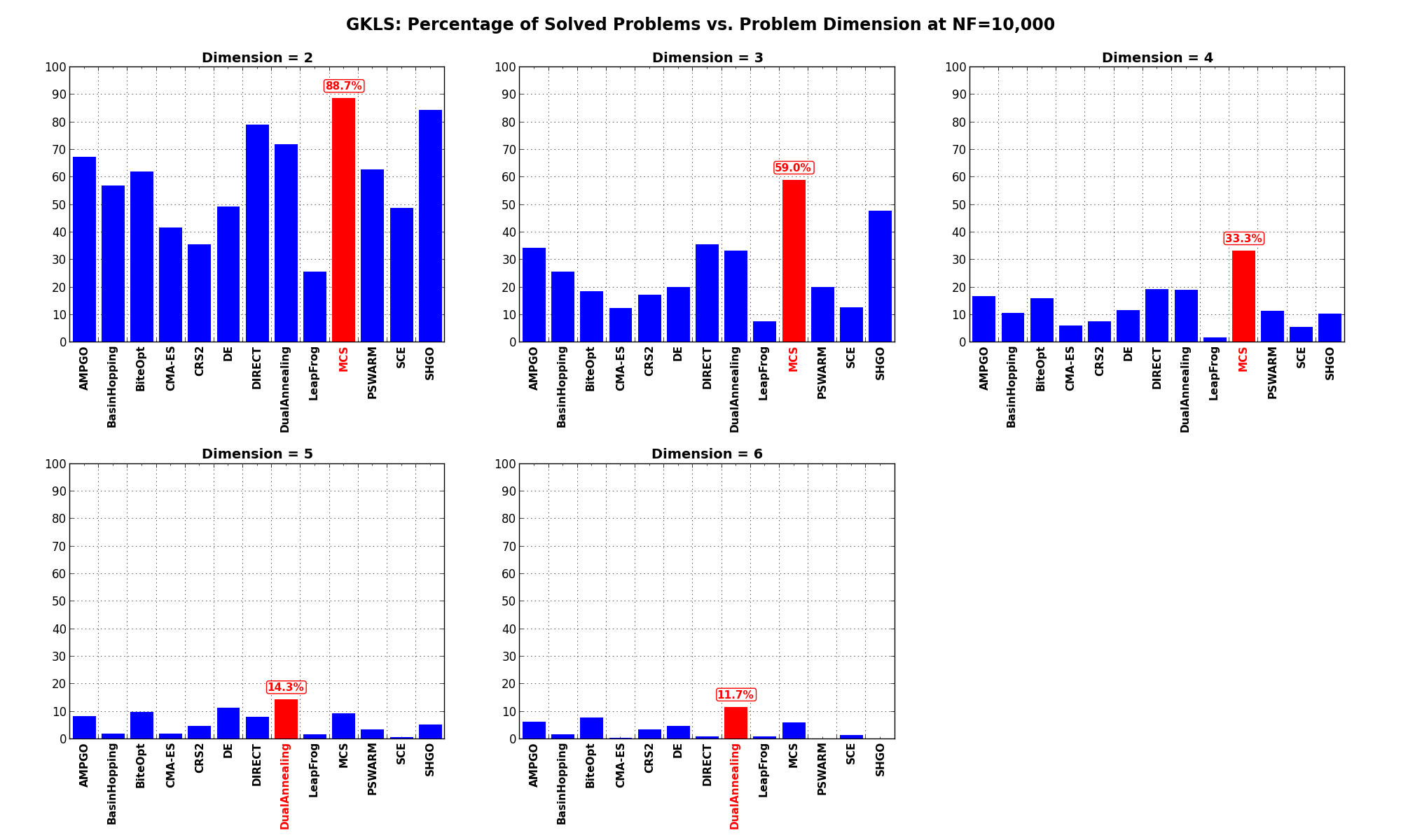
Percentage of problems solved as a function of problem dimension at :math:`NF = 10,000`

Figure 2.8: Percentage of problems solved as a function of problem dimension for the GKLS test suite at $NF = 10,000$

GKLS¶

Methodology¶

General Solvers Performances¶

Sensitivities on Functions Evaluations Budget¶

Dimensionality Effects¶

Table Of Contents

Previous topic

Next topic

This Page

Navigation

GKLS¶

Methodology¶

General Solvers Performances¶

Sensitivities on Functions Evaluations Budget¶

Dimensionality Effects¶

Table Of Contents

Previous topic

Next topic

This Page

Quick search

Navigation