N-D Test Functions H¶

class go_benchmark.Hansen(dimensions=2)¶

Hansen test objective function.

This class defines the Hansen global optimization problem. This is a multimodal minimization problem defined as follows:

$f_{\text{Hansen}}(\mathbf{x}) = \left[ \sum_{i=0}^4(i+1)\cos(ix_1+i+1)\right ] \left[\sum_{j=0}^4(j+1)\cos[(j+2)x_2+j+1])\right ]$

Here, $n$ represents the number of dimensions and $x_i \in [-10, 10]$ for $i=1,2$ .

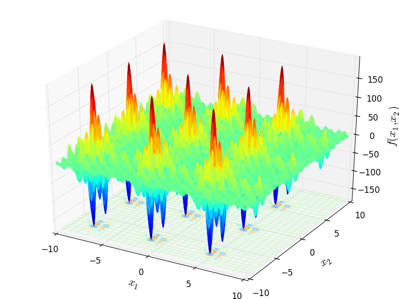
Two-dimensional Hansen function

Global optimum: $f(x_i) = -2.3458$ for $\mathbf{x} = [-7.58989583, -7.70831466]$ .

class go_benchmark.Hartmann3(dimensions=3)¶

Hartmann3 test objective function.

This class defines the Hartmann3 global optimization problem. This is a multimodal minimization problem defined as follows:

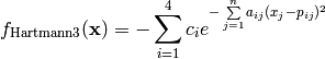
$f_{\text{Hartmann3}}(\mathbf{x}) = -\sum\limits_{i=1}^{4} c_i e^{-\sum\limits_{j=1}^{n}a_{ij}(x_j - p_{ij})^2}$

Where, in this exercise:

$\begin{array}{l|ccc|c|ccr} \hline i & & a_{ij}& & c_i & & p_{ij} & \\ \hline 1 & 3.0 & 10.0 & 30.0 & 1.0 & 0.689 & 0.1170 & 0.2673 \\ 2 & 0.1 & 10.0 & 35.0 & 1.2 & 0.4699 & 0.4387 & 0.7470 \\ 3 & 3.0 & 10.0 & 30.0 & 3.0 & 0.1091 & 0.8732 & 0.5547 \\ 4 & 0.1 & 10.0 & 35.0 & 3.2 & 0.0381 & 0.5743 & 0.8828 \\ \hline \end{array}$

Here, $n$ represents the number of dimensions and $x_i \in [0, 1]$ for $i=1,2,3$ .

Global optimum: $f(x_i) = -3.86278214782076$ for $\mathbf{x} = [0.1, 0.55592003, 0.85218259]$

class go_benchmark.Hartmann6(dimensions=6)¶

Hartmann6 test objective function.

This class defines the Hartmann6 global optimization problem. This is a multimodal minimization problem defined as follows:

$f_{\text{Hartmann6}}(\mathbf{x}) = -\sum\limits_{i=1}^{4} c_i e^{-\sum\limits_{j=1}^{n}a_{ij}(x_j - p_{ij})^2}$

Where, in this exercise:

$\begin{array}{l|cccccc|r} \hline i & & & a_{ij} & & & & c_i \\ \hline 1 & 10.0 & 3.0 & 17.0 & 3.50 & 1.70 & 8.00 & 1.0 \\ 2 & 0.05 & 10.0 & 17.0 & 0.10 & 8.00 & 14.00 & 1.2 \\ 3 & 3.00 & 3.50 & 1.70 & 10.0 & 17.00 & 8.00 & 3.0 \\ 4 & 17.00 & 8.00 & 0.05 & 10.00 & 0.10 & 14.00 & 3.2 \\ \hline \end{array} \newline \\ \newline \begin{array}{l|cccccr} \hline i & & & p_{ij} & & & \\ \hline 1 & 0.1312 & 0.1696 & 0.5569 & 0.0124 & 0.8283 & 0.5886 \\ 2 & 0.2329 & 0.4135 & 0.8307 & 0.3736 & 0.1004 & 0.9991 \\ 3 & 0.2348 & 0.1451 & 0.3522 & 0.2883 & 0.3047 & 0.6650 \\ 4 & 0.4047 & 0.8828 & 0.8732 & 0.5743 & 0.1091 & 0.0381 \\ \hline \end{array}$

Here, $n$ represents the number of dimensions and $x_i \in [0, 1]$ for $i=1,...,6$ .

Global optimum: $f(x_i) = -3.32236801141551$ for $\mathbf{x} = [0.20168952, 0.15001069, 0.47687398, 0.27533243, 0.31165162, 0.65730054]$

class go_benchmark.HelicalValley(dimensions=3)¶

HelicalValley test objective function.

This class defines the HelicalValley global optimization problem. This is a multimodal minimization problem defined as follows:

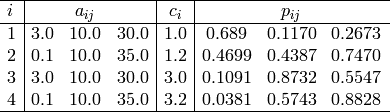
$f_{\text{HelicalValley}}(\mathbf{x}) = 100{[z-10\Psi(x_1,x_2)]^2+(\sqrt{x_1^2+x_2^2}-1)^2}+x_3^2$

Where, in this exercise:

$2\pi\Psi(x,y) = \begin{cases} \arctan(y/x) & \textrm{for} x > 0 \\ \pi + \arctan(y/x) & \textrm{for} x < 0 \end{cases}$

Here, $n$ represents the number of dimensions and $x_i \in [-\infty, \infty]$ for $i=1,2,3$ .

Global optimum: $f(x_i) = 0$ for $\mathbf{x} = [1, 0, 0]$

class go_benchmark.HimmelBlau(dimensions=2)¶

HimmelBlau test objective function.

This class defines the HimmelBlau global optimization problem. This is a multimodal minimization problem defined as follows:

$f_{\text{HimmelBlau}}(\mathbf{x}) = (x_1^2 + x_2 - 11)^2 + (x_1 + x_2^2 -7)^2$

Here, $n$ represents the number of dimensions and $x_i \in [-6, 6]$ for $i=1,2$ .

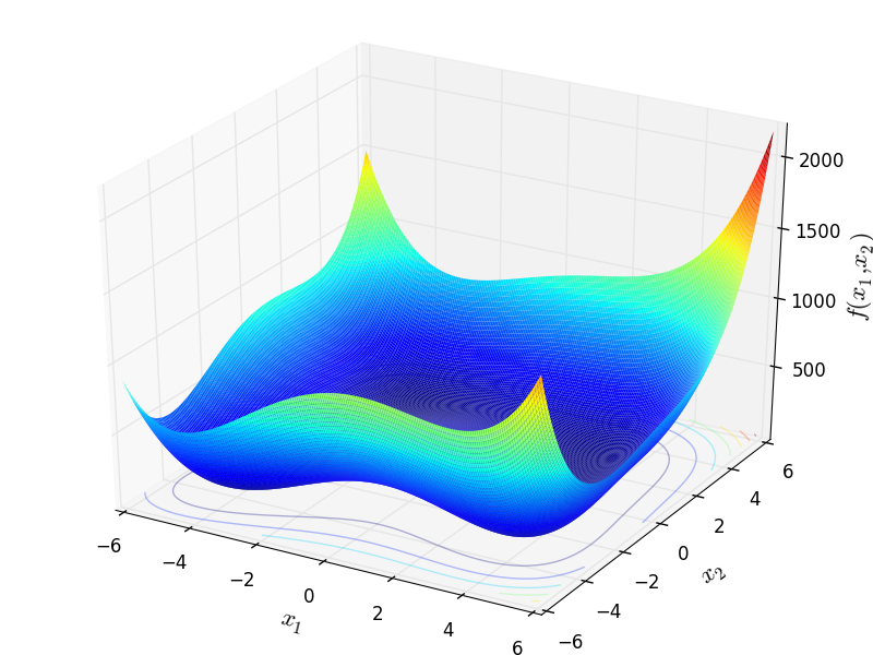
Two-dimensional HimmelBlau function

Global optimum: $f(x_i) = 0$ for $\mathbf{x} = [0, 0]$

class go_benchmark.HolderTable(dimensions=2)¶

HolderTable test objective function.

This class defines the HolderTable global optimization problem. This is a multimodal minimization problem defined as follows:

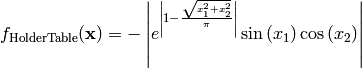
$f_{\text{HolderTable}}(\mathbf{x}) = - \left|{e^{\left|{1 - \frac{\sqrt{x_{1}^{2} + x_{2}^{2}}}{\pi} }\right|} \sin\left(x_{1}\right) \cos\left(x_{2}\right)}\right|$

Here, $n$ represents the number of dimensions and $x_i \in [-10, 10]$ for $i=1,2$ .

Two-dimensional HolderTable function

Global optimum: $f(x_i) = -19.20850256788675$ for $x_i = \pm 9.664590028909654$ for $i=1,2$

class go_benchmark.Holzman(dimensions=3)¶

Holzman test objective function.

This class defines the Holzman global optimization problem. This is a multimodal minimization problem defined as follows:

$f_{\text{Holzman}}(\mathbf{x}) = \sum_{i=0}^{99} \left [ e^{\frac{1}{x_1} (u_i-x_2)^{x_3}} -0.1(i+1) \right ]$

Where, in this exercise:

$u_i = 25 + (-50 \log{[0.01(i+1)]})^{2/3}$

Here, $n$ represents the number of dimensions and $x_1 \in [0, 100], x_2 \in [0, 25.6], x_3 \in [0, 5]$ .

Global optimum: $f(x_i) = 0$ for $\mathbf{x} = [50, 25, 1.5]$

class go_benchmark.Hosaki(dimensions=2)¶

Hosaki test objective function.

This class defines the Hosaki global optimization problem. This is a multimodal minimization problem defined as follows:

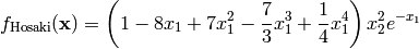
$f_{\text{Hosaki}}(\mathbf{x}) = \left ( 1 - 8x_1 + 7x_1^2 - \frac{7}{3}x_1^3 + \frac{1}{4}x_1^4 \right )x_2^2e^{-x_1}$

Here, $n$ represents the number of dimensions and $x_i \in [0, 10]$ for $i=1,2$ .

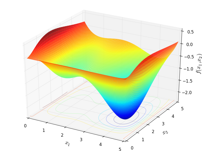
Two-dimensional Hosaki function

Global optimum: $f(x_i) = -2.3458$ for $\mathbf{x} = [4, 2]$ .

N-D Test Functions H¶

Previous topic

Next topic

This Page

Navigation

N-D Test Functions H¶

Previous topic

Next topic

This Page

Quick search

Navigation