AMPGO stands for Adaptive Memory Programming for Global Optimization, and its detailed implementation is described in the paper “Adaptive Memory Programming for Constrained Global Optimization” located here:
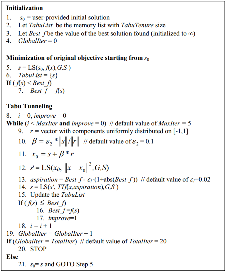
The following figure provides a pseudo-code description of the Tabu Tunneling algorithm, which is the basis of the global search in AMPGO:

AMPGO Pseudo code - tabu tunnelling algorithm
 AMPGO Function Signature in Python
The call signature of AMPGO‘s Python implementation follows very closely the standard signature for the minimization functions in the scipy.optimize package in scipy.
Finds the global minimum of a function using the AMPGO (Adaptive Memory Programming for Global Optimization) algorithm.
| Parameters: |
|
|---|---|
| Returns: | A tuple of 5 elements, in the following order:
|
| Return type: | tuple |
 Sensitivities on the AMPGO Input Parameters
This sections presents a number of sensitivities on the AMPGO input parameters, which may be helpful in guiding the choice of the parameters themselves depending on the difficulty of the optimization problem at hand. The most fundamental argument is evidently the local solver, followed by the maximum number of Tabu Tunnelling iterations allowed and the length of the list containing the “tabu points” (i.e., the previous local minima found by the method).
The AMPGO Python implementation supports a number of local solvers, from scipy and OpenOpt . The available solvers can be categorized as follows:
| Scipy Solver | Description |
|---|---|
| Nelder-Mead | Downhill Simplex algorithm |
| L-BFGS-B | L-BFGS-B algorithm |
| Powell | Powell’s conjugate direction method |
| SLSQP | Sequential Least Squares Programming |
| TNC | Truncated Newton algorithm |
| OpenOpt Solver | Description |
|---|---|
| AUGLAG | Augmented Lagrangian method |
| BOBYQA | Powell’s derivative-free method |
| MMA | Method of moving asymptotes |
| PTN | Preconditioned truncated Newton method |
| RALG | R-algorithm with adaptive space dilation |
| SLMVM2 | Shifted limited-memory variable-metric |
| SQLCP | Sequential Quadratic Programming |
I applied AMPGO to the entire benchmark suite of N-D optimization problems, considering for every benchmark function 100 random starting points. As there are currently 12 local solvers supported by AMPGO, I re-run the same suite 12 times changing the local solver.
The results obtained are shown in the following table:
| Optimization Method | Overall Success (%) | Functions Evaluations |
|---|---|---|
| AUGLAG | 57.957 | 1633 |
| BOBYQA | 70.418 | 813 |
| L-BFGS-B | 79.027 | 611 |
| MMA | 57.489 | 1656 |
| Nelder-Mead | 65.587 | 1008 |
| Powell | 63.636 | 1248 |
| PTN | 60.777 | 1042 |
| RALG | 64.565 | 952 |
| SLMVM2 | 67.054 | 861 |
| SLSQP | 65.484 | 3039 |
| SQLCP | 46.902 | 1231 |
| TNC | 63.804 | 861 |
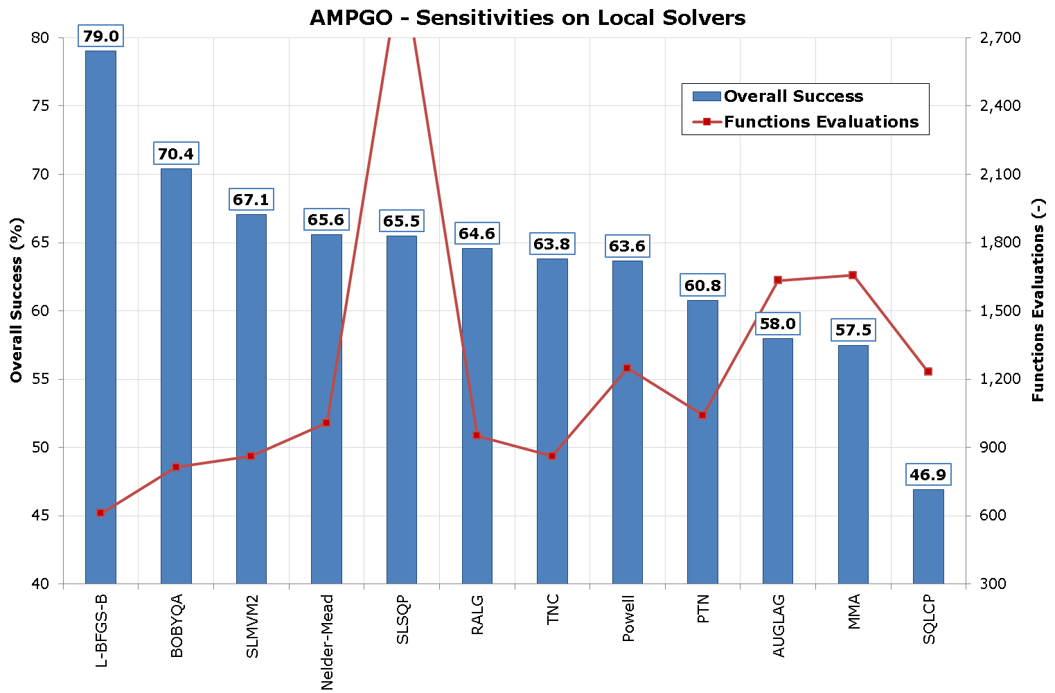
So, for example, AMPGO with L-BFGS-B local solver was able to solve, on average, 79.0% of all the test functions for all the 100 random starting points using, on average, 611 functions evaluations. This is also shown graphically in the picture below.

AMPGO - Local solvers sensitivity
One of the parameters you can supply to the AMPGO optimization routine is the maximum number of Tabu Tunnelling iterations allowed during each global iteration (maxiter). Once a local minimum is found, AMPGO will start a Tunnelling phase to try and move away from this local optimum; if no better point is found, it will start again from another point and try to move away from this local minimum. It will do so for maxiter times.
The table below highlights the various experiments I have run by applying AMPGO to the entire benchmark suite of N-D optimization problems, considering for every benchmark function 100 random starting points. The maxiter parameter has been allowed to range between 1 and 8, but the results are inconclusive: 2 seems to be the absolute minimum to get a higher level of global convergence, but then there isn’t much of a difference between choosing maxiter=3 and maxiter=8.
The results obtained are shown in the following table:
| Tabu Tunnelling Phases | Overall Success (%) | Functions Evaluations |
|---|---|---|
| 1 | 76.783 | 635 |
| 2 | 78.837 | 607 |
| 3 | 78.875 | 615 |
| 4 | 78.685 | 619 |
| 5 | 79.027 | 611 |
| 6 | 78.864 | 625 |
| 7 | 78.750 | 623 |
| 8 | 78.647 | 635 |
The results appear slightly more interesting if we remove from the analysis all the N-D benchmark functions for which AMPGO achieved global convergence irrespectively of the number of Tabu Tunnelling phases. This information is condensed in the following table:
| Tabu Tunnelling Phases | Overall Success (%) | Functions Evaluations |
|---|---|---|
| 1 | 49.143 | 1319 |
| 2 | 53.643 | 1256 |
| 3 | 53.726 | 1274 |
| 4 | 53.310 | 1281 |
| 5 | 54.060 | 1262 |
| 6 | 53.702 | 1292 |
| 7 | 53.452 | 1288 |
| 8 | 53.226 | 1315 |
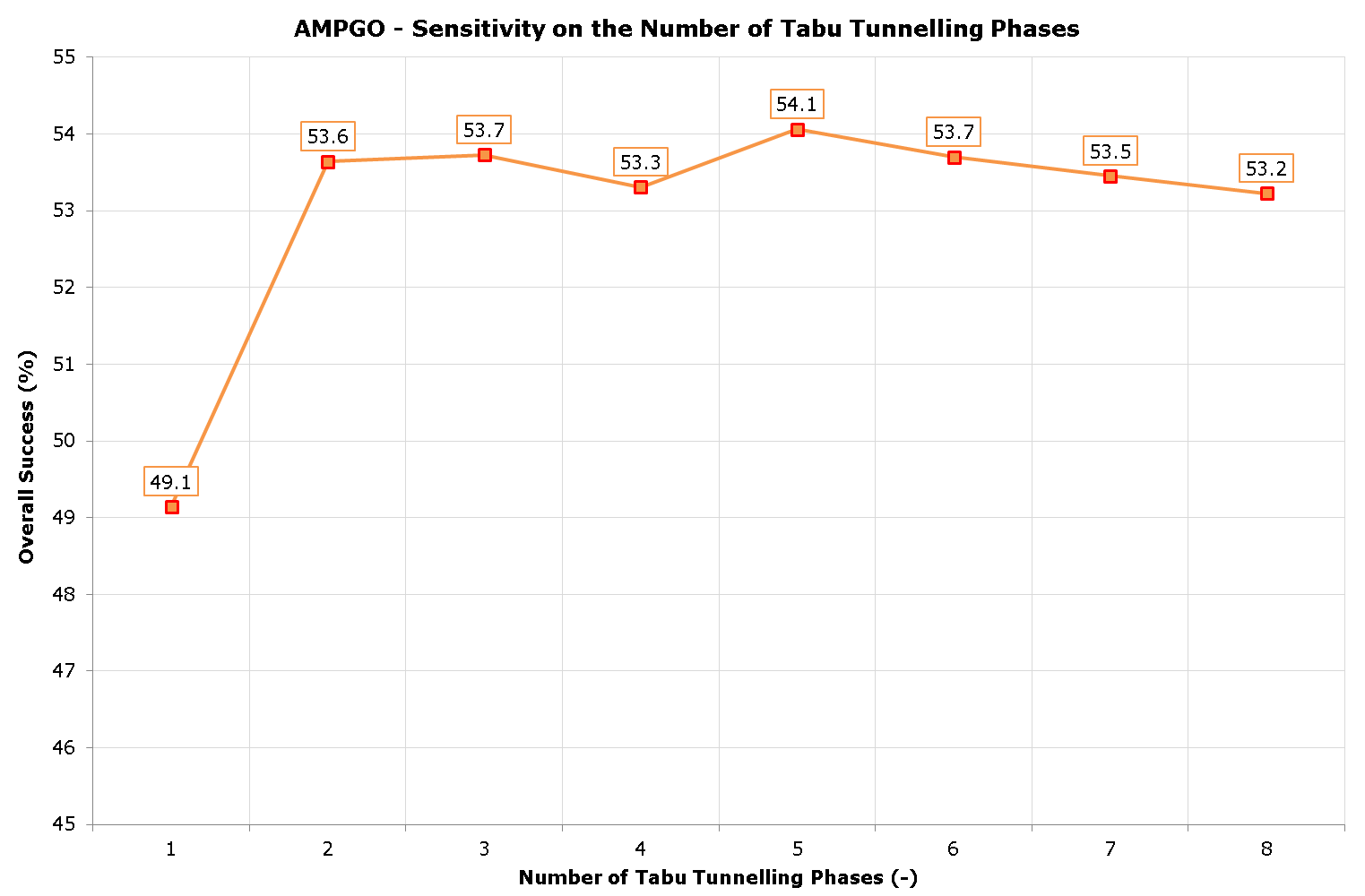
The above results are also shown graphically in the next figure; all in all, the default choice of maxiter=5 in the AMPGO code appears to be a sensible one.

AMPGO - Number of tabu tunnelling phases sensitivity
Another parameter you can supply to the AMPGO optimization routine is the maximum size of the Tabu List, which is a list containing the latest tabulistsize local minima found by the optimizer. This is a list of points from which to move away, including both the most recent local solution of the original minimization problem, and recent solutions of tunneling sub-problems which failed to achieve the desired condition.
The table below highlights the various experiments I have run by applying AMPGO to the entire benchmark suite of N-D optimization problems, considering for every benchmark function 100 random starting points.
The tabulistsize parameter has been allowed to range between 2 and 8, but again the results are inconclusive: There appear to be little difference between choosing 2 over 8, even though for real-life problems (with many local minima) I would suggest to keep the tabulistsize number greater than 2.
The results obtained are shown in the following table:
| Tabu List Size | Overall Success (%) | Functions Evaluations |
|---|---|---|
| 2 | 77.272 | 633 |
| 3 | 78.652 | 626 |
| 4 | 78.880 | 618 |
| 5 | 79.027 | 611 |
| 6 | 79.190 | 620 |
| 7 | 79.114 | 617 |
| 8 | 79.527 | 604 |
Again, removing from the analysis all the N-D benchmark functions for which AMPGO achieved global convergence irrespectively of the size of the tabu list shows some more interesting trend, as depicted in the following table:
| Tabu List Size | Overall Success (%) | Functions Evaluations |
|---|---|---|
| 2 | 53.011 | 1243 |
| 3 | 55.865 | 1232 |
| 4 | 56.337 | 1217 |
| 5 | 56.640 | 1202 |
| 6 | 56.978 | 1223 |
| 7 | 56.820 | 1215 |
| 8 | 57.674 | 1190 |
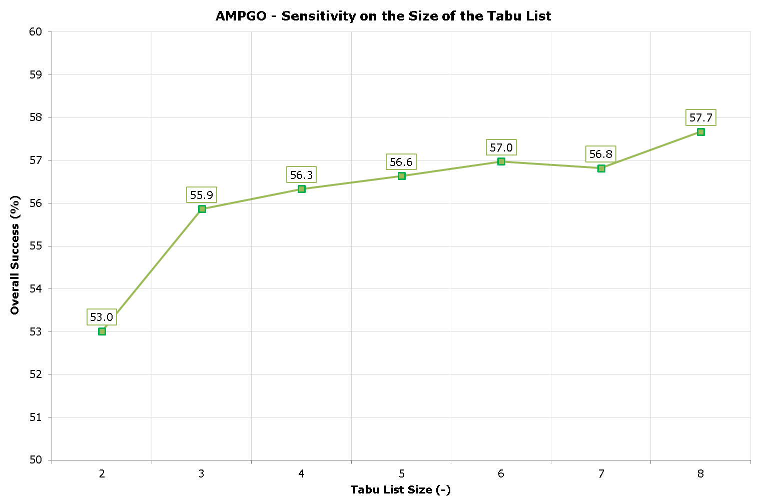
The above results are also shown graphically in the next figure; all in all, it appears that choosing a high enough size of the tabu list slightly improves the optimization results.

AMPGO - Size of the tabu list sensitivity
Another parameter you can supply to the AMPGO optimization routine is the Tabu List strategy, which is the strategy to use when the size of the tabu list exceeds tabulistsize. It can be ‘oldest’ to drop the oldest point from the tabu list or ‘farthest’ to drop the element farthest from the last local minimum found.
The table below highlights the various experiments I have run by applying AMPGO to the entire benchmark suite of N-D optimization problems, considering for every benchmark function 100 random starting points.
The tabustrategy parameter has been allowed to range between ‘oldest’ and ‘farthest’.
The results obtained are shown in the following table:
| Tabu Strategy | Overall Success (%) | Functions Evaluations |
|---|---|---|
| farthest | 79.027 | 611 |
| oldest | 78.750 | 630 |
This time, removing from the analysis all the N-D benchmark functions for which AMPGO achieved global convergence irrespectively of the tabustrategy value shows very little difference between the two strategies, so any user’s choice should be sensible in this respect.
| Tabu Strategy | Overall Success (%) | Functions Evaluations |
|---|---|---|
| farthest | 50.526 | 1347 |
| oldest | 49.872 | 1390 |