Navigation
- index
- next |
- previous |

- Home »
- The Benchmarks »
- LGMVG
 LGMVG
| Fopt Known | Xopt Known | Difficulty |
|---|---|---|
| Yes | No | Easy |
The LGMVG test suite is a Gaussian landscape generator and it is intended to be a general-purpose tool for generating unconstrained single-objective continuous test problems within box-bounded search spaces. The implementation follows the “Max-Set of Gaussians Landscape Generator” described in http://boyuan.global-optimization.com/LGMVG/index.htm .
The major motivation for this problem generator was to increase the research value of experimental studies on Evolutionary Algorithms and other optimization algorithms by giving experimenters access to a set of purposefully built test problems with controllable internal structure.
The major advantages of using a landscape generator compared to using classical benchmark test problems are listed as below:
 Methodology
The basic components or building-blocks of this landscape generator are a set of multivariate Gaussian functions:
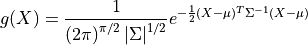
Where  is an
is an  -dimenional vector of means and
  is a
is a  covariance matrix.
The fitness value of a vector
covariance matrix.
The fitness value of a vector  is determined by the weighted component that gives it the largest value:
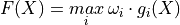
Since the normalizing factor of each Gaussian function is a constant, it can be combined with its weight  .
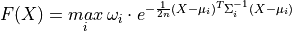
Also, the -th root of the Gaussian function (i.e., is the dimensionality) is used to avoid some issues in high-dimensional spaces.
The actual fitness function has the following form:
.
Also, the -th root of the Gaussian function (i.e., is the dimensionality) is used to avoid some issues in high-dimensional spaces.
The actual fitness function has the following form:
Generally speaking, the number of components serves as a rough indicator of the multimodality of the generated landscapes. However, the actual number of optima is likely to be less than the number of components as the peaks of weak components could be dominated by others.
That said, my approach to generate test functions for this benchmark has been the following:
 and
and  is generated either from a uniform distribution or from a normal distribution is either a random number between 0 and 1 or a specific array used to explicitly control the height of each component
With all these variable settings, I generated 76 valid test function per dimension, thus the current LGMVG test suite contains 304 benchmark functions.
A few examples of 2D benchmark functions created with the LGMVG generator can be seen in Figure 7.1.
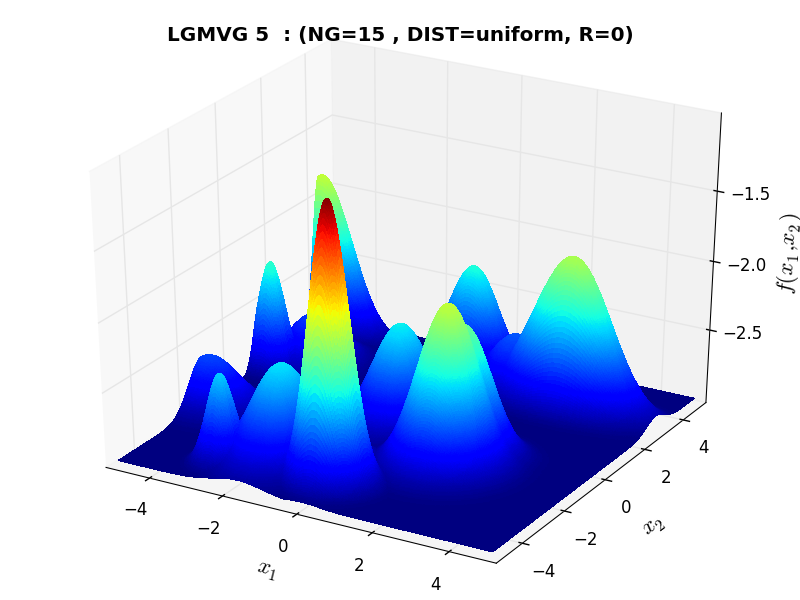
LGMVG Function 5 |
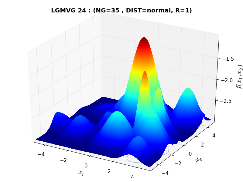
LGMVG Function 24 |
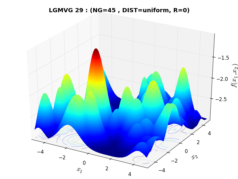
LGMVG Function 29 |
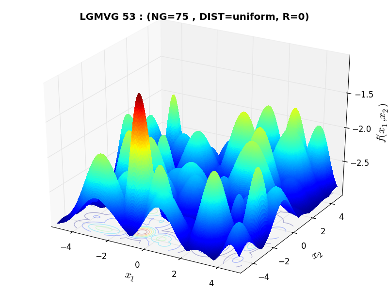
LGMVG Function 53 |
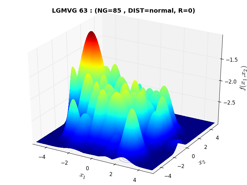
LGMVG Function 63 |
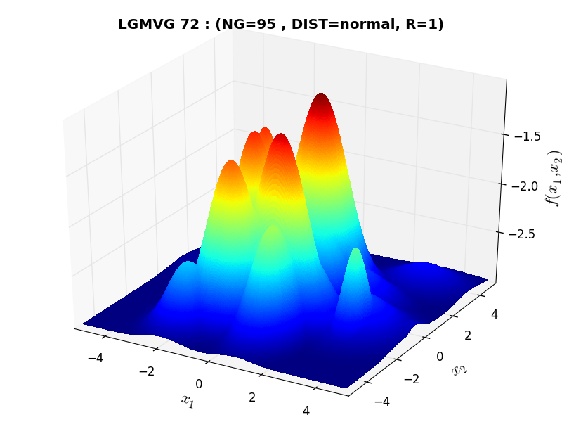
LGMVG Function 72 |
 General Solvers Performances
Table 7.1 below shows the overall success of all Global Optimization algorithms, considering every benchmark function,
for a maximum allowable budget of  .
.
The LGMVG benchmark suite is a relatively easy test suite: the best solver for is SHGO, with a success
rate of 77.6%, closely followed by DualAnnealing and MCS.
Note
The reported number of functions evaluations refers to successful optimizations only.
| Optimization Method | Overall Success (%) | Functions Evaluations |
|---|---|---|
| AMPGO | 46.38% | 570 |
| BasinHopping | 13.16% | 339 |
| BiteOpt | 43.75% | 486 |
| CMA-ES | 28.29% | 623 |
| CRS2 | 50.66% | 1,002 |
| DE | 42.11% | 1,198 |
| DIRECT | 65.79% | 375 |
| DualAnnealing | 75.33% | 322 |
| LeapFrog | 32.57% | 246 |
| MCS | 70.07% | 488 |
| PSWARM | 20.39% | 1,686 |
| SCE | 48.36% | 604 |
| SHGO | 77.63% | 427 |
These results are also depicted in Figure 7.2, which shows that SHGO is the better-performing optimization algorithm, followed by DualAnnealing and MCS.
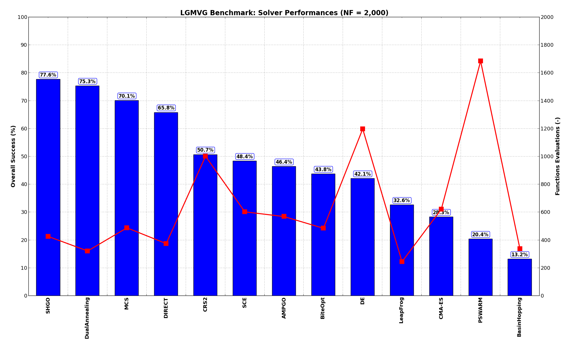
Figure 7.2: Optimization algorithms performances on the LGMVG test suite at
Pushing the available budget to a very generous  , the results show SHGO basically solving the vast
majority of problems (more than 95%), followed at a distance by MCS and DualAnnealing. The results are also
shown visually in Figure 7.3.
, the results show SHGO basically solving the vast
majority of problems (more than 95%), followed at a distance by MCS and DualAnnealing. The results are also
shown visually in Figure 7.3.
| Optimization Method | Overall Success (%) | Functions Evaluations |
|---|---|---|
| AMPGO | 73.03% | 2,304 |
| BasinHopping | 11.84% | 412 |
| BiteOpt | 49.67% | 1,072 |
| CMA-ES | 33.22% | 1,390 |
| CRS2 | 57.57% | 1,194 |
| DE | 69.08% | 2,113 |
| DIRECT | 73.68% | 791 |
| DualAnnealing | 79.61% | 492 |
| LeapFrog | 32.57% | 246 |
| MCS | 86.18% | 1,214 |
| PSWARM | 57.89% | 2,138 |
| SCE | 53.62% | 896 |
| SHGO | 95.07% | 1,357 |
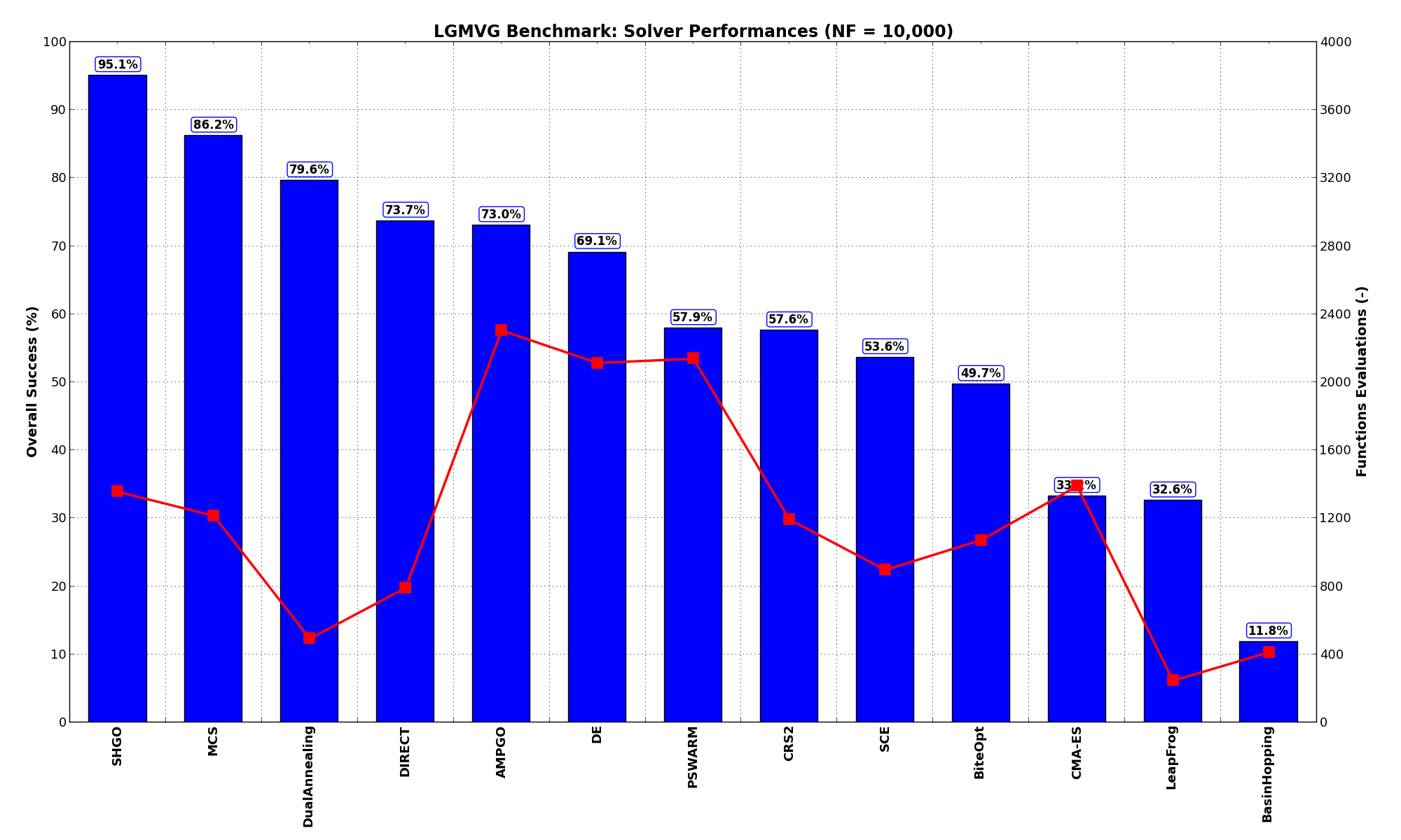
Figure 7.3: Optimization algorithms performances on the LGMVG test suite at
 Sensitivities on Functions Evaluations Budget
It is also interesting to analyze the success of an optimization algorithm based on the fraction (or percentage) of problems solved given a fixed number of allowed function evaluations, let’s say 100, 200, 300,... 2000, 5000, 10000.
In order to do that, we can present the results using two different types of visualizations. The first one is some sort of “small multiples” in which each solver gets an individual subplot showing the improvement in the number of solved problems as a function of the available number of function evaluations - on top of a background set of grey, semi-transparent lines showing all the other solvers performances.
This visual gives an indication of how good/bad is a solver compared to all the others as function of the budget available. Results are shown in Figure 7.4.
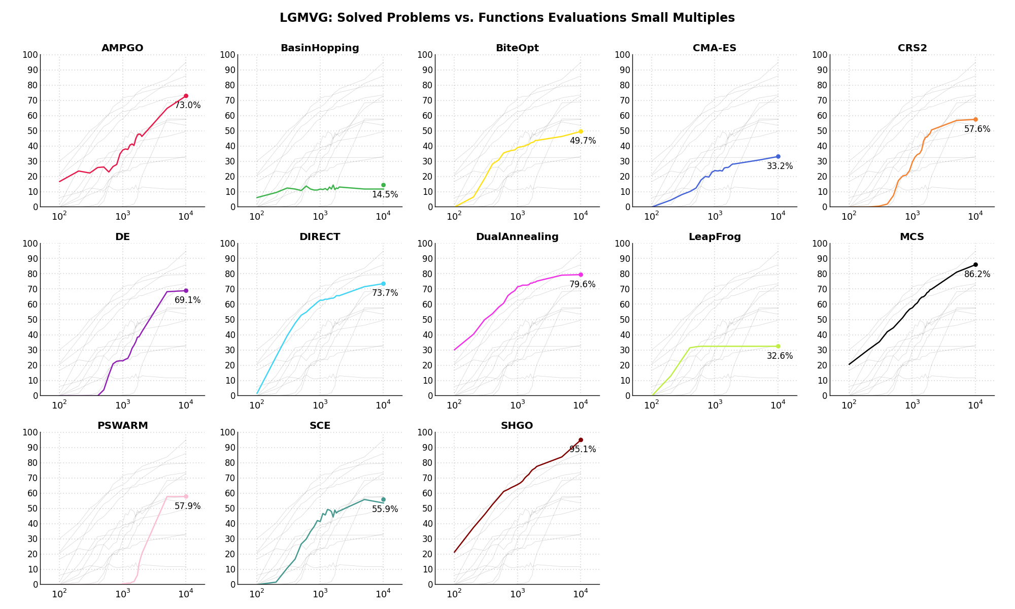
Figure 7.4: Percentage of problems solved given a fixed number of function evaluations on the LGMVG test suite
The second type of visualization is sometimes referred as “Slopegraph” and there are many variants on the plot layout and appearance that we can implement. The version shown in Figure 7.5 aggregates all the solvers together, so it is easier to spot when a solver overtakes another or the overall performance of an algorithm while the available budget of function evaluations changes.
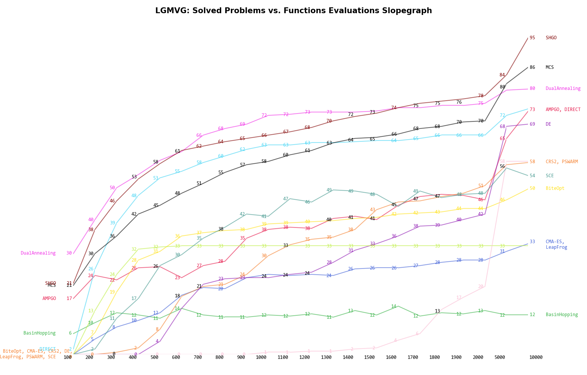
Figure 7.5: Percentage of problems solved given a fixed number of function evaluations on the LGMVG test suite
A few obvious conclusions we can draw from these pictures are:
 Dimensionality Effects
Since I used the LGMVG test suite to generate test functions with dimensionality ranging from 2 to 5, it is interesting to take a look at the solvers performances as a function of the problem dimensionality. Of course, in general it is to be expected that for larger dimensions less problems are going to be solved - although it is not always necessarily so as it also depends on the function being generated. Results are shown in Table 7.3 .
| Solver | N = 2 | N = 3 | N = 4 | N = 5 | Overall |
|---|---|---|---|---|---|
| AMPGO | 82.9 | 53.9 | 32.9 | 15.8 | 46.4 |
| BasinHopping | 19.7 | 18.4 | 9.2 | 5.3 | 13.2 |
| BiteOpt | 85.5 | 47.4 | 30.3 | 11.8 | 43.8 |
| CMA-ES | 48.7 | 25.0 | 21.1 | 18.4 | 28.3 |
| CRS2 | 85.5 | 59.2 | 44.7 | 13.2 | 50.7 |
| DE | 92.1 | 71.1 | 5.3 | 0.0 | 42.1 |
| DIRECT | 98.7 | 80.3 | 60.5 | 23.7 | 65.8 |
| DualAnnealing | 100.0 | 77.6 | 67.1 | 56.6 | 75.3 |
| LeapFrog | 59.2 | 30.3 | 17.1 | 23.7 | 32.6 |
| MCS | 98.7 | 89.5 | 56.6 | 35.5 | 70.1 |
| PSWARM | 80.3 | 1.3 | 0.0 | 0.0 | 20.4 |
| SCE | 82.9 | 48.7 | 27.6 | 34.2 | 48.4 |
| SHGO | 100.0 | 98.7 | 77.6 | 34.2 | 77.6 |
Figure 7.6 shows the same results in a visual way.
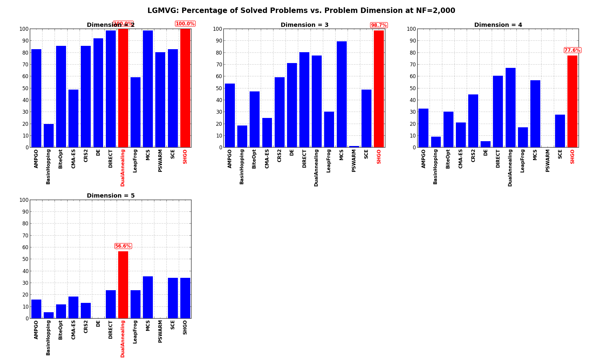
Figure 7.6: Percentage of problems solved as a function of problem dimension for the LGMVG test suite at
What we can infer from the table and the figure is that, for lower dimensionality problems ( ), the SHGO
algorithm has a significant advantage over all other algorithms, although the SciPy optimizer DualAnnealing is not
too far behind. For higher dimensionality problems (
), the SHGO
algorithm has a significant advantage over all other algorithms, although the SciPy optimizer DualAnnealing is not
too far behind. For higher dimensionality problems ( ), DualAnnealing appears to be better than any other solver.
Pushing the available budget to a very generous , the results show that SHGO is always the best solver
no matter what dimensionality we are considering. It has 100% success rate for low dimensional problems ( )
and very good convergence results for higher dimensions.
)
and very good convergence results for higher dimensions.
The results for the benchmarks at are displayed in Table 7.4 and Figure 7.7.
| Solver | N = 2 | N = 3 | N = 4 | N = 5 | Overall |
|---|---|---|---|---|---|
| AMPGO | 100.0 | 86.8 | 63.2 | 42.1 | 73.0 |
| BasinHopping | 21.1 | 14.5 | 6.6 | 5.3 | 11.8 |
| BiteOpt | 90.8 | 57.9 | 34.2 | 15.8 | 49.7 |
| CMA-ES | 61.8 | 27.6 | 23.7 | 19.7 | 33.2 |
| CRS2 | 85.5 | 61.8 | 47.4 | 35.5 | 57.6 |
| DE | 92.1 | 75.0 | 57.9 | 51.3 | 69.1 |
| DIRECT | 100.0 | 84.2 | 68.4 | 42.1 | 73.7 |
| DualAnnealing | 100.0 | 81.6 | 73.7 | 63.2 | 79.6 |
| LeapFrog | 59.2 | 30.3 | 17.1 | 23.7 | 32.6 |
| MCS | 98.7 | 97.4 | 88.2 | 60.5 | 86.2 |
| PSWARM | 97.4 | 61.8 | 42.1 | 30.3 | 57.9 |
| SCE | 84.2 | 59.2 | 40.8 | 30.3 | 53.6 |
| SHGO | 100.0 | 100.0 | 90.8 | 89.5 | 95.1 |
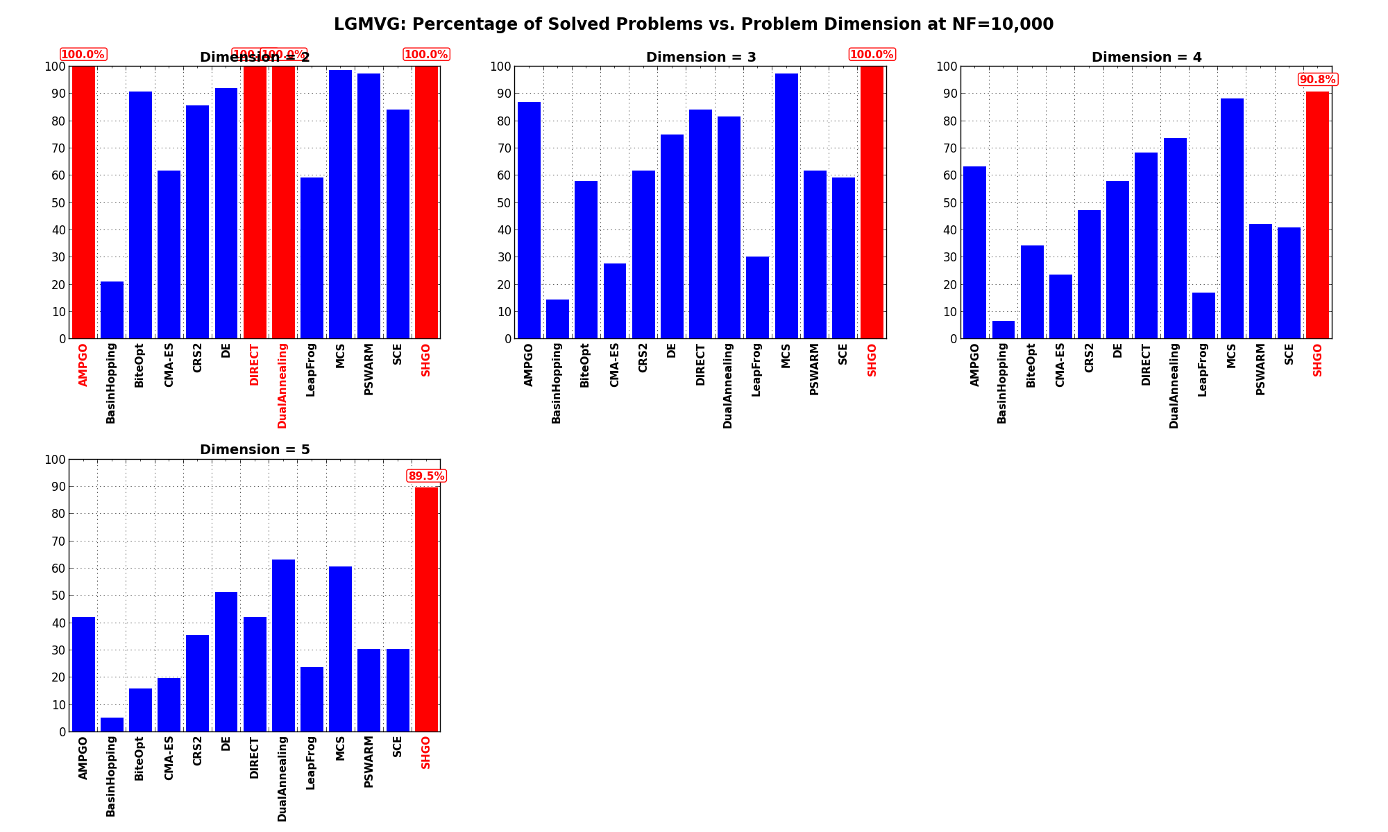
Figure 7.7: Percentage of problems solved as a function of problem dimension for the LGMVG test suite at