GlobalLib

Fopt Known	Xopt Known	Difficulty
Yes	Yes	Easy

Arnold Neumaier maintains a suite of test problems termed “COCONUT Benchmark” and Sahinidis has converted the GlobalLib and PricentonLib AMPL/GAMS dataset into C/Fortran code (http://archimedes.cheme.cmu.edu/?q=dfocomp ). From Sahinidis’ work I have taken the C files - which are not a model of programming as they were automatically translated from GAMS models - and used a simple C parser to convert the benchmarks from C to Python.

The automatic conversion generated a Python module that is 27,400 lines long, and trust me, you don’t want to go through it and look at the objective functions definitions...

The global minima are taken from Sahinidis or from Neumaier or refined using the NEOS server when the accuracy of the reported minima is too low. The suite contains 181 test functions with dimensionality varying between 2 and 9.

Methodology

There isn’t much to describe in terms of methodology, as everything has been automatically translated from C files to Python. Some of the 2D objective functions in this benchmark test suite can be seen in Figure 12.1.

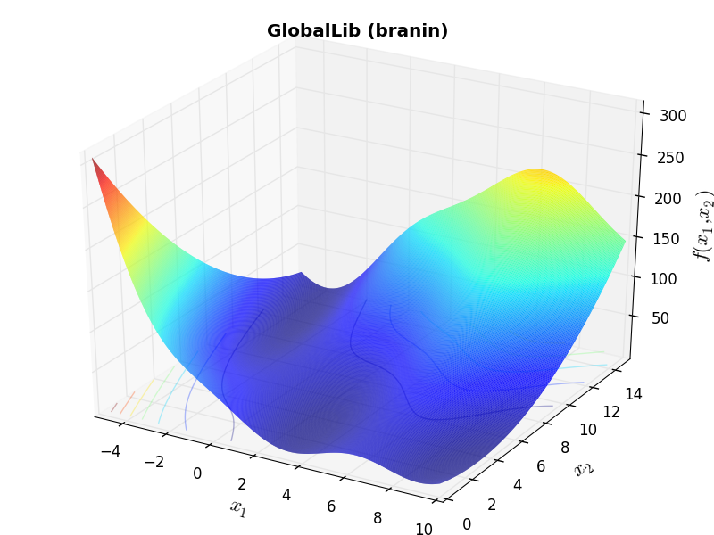
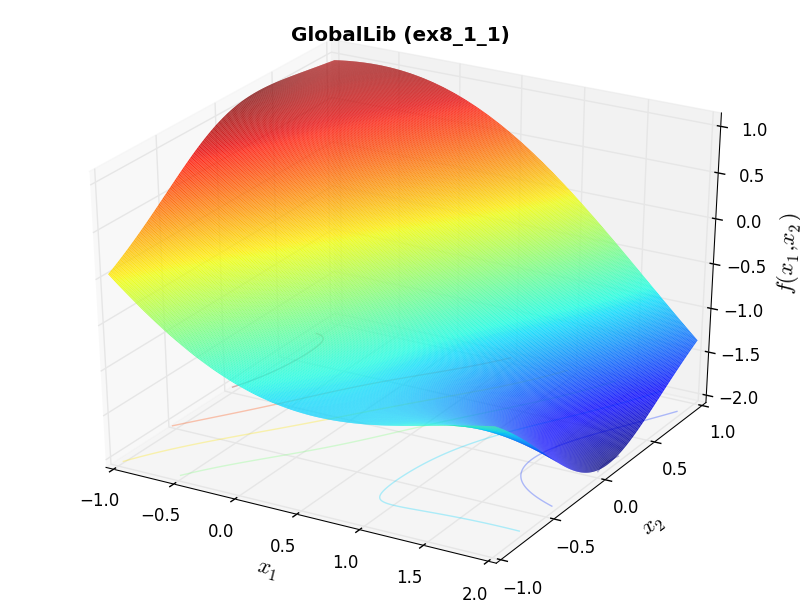
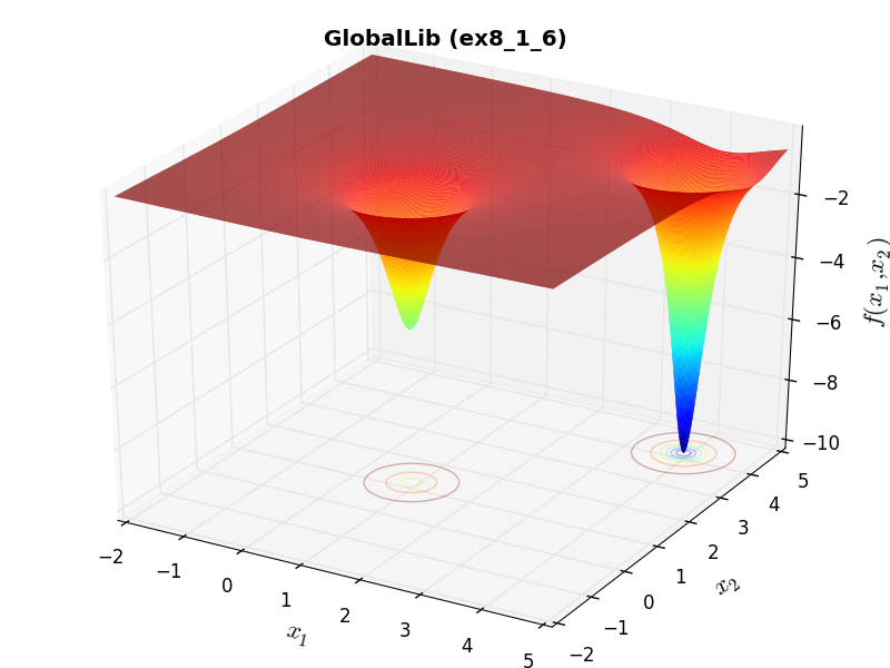
GlobalLib Function Branin	GlobalLib Function ex8_1_1	GlobalLib Function ex8_1_6
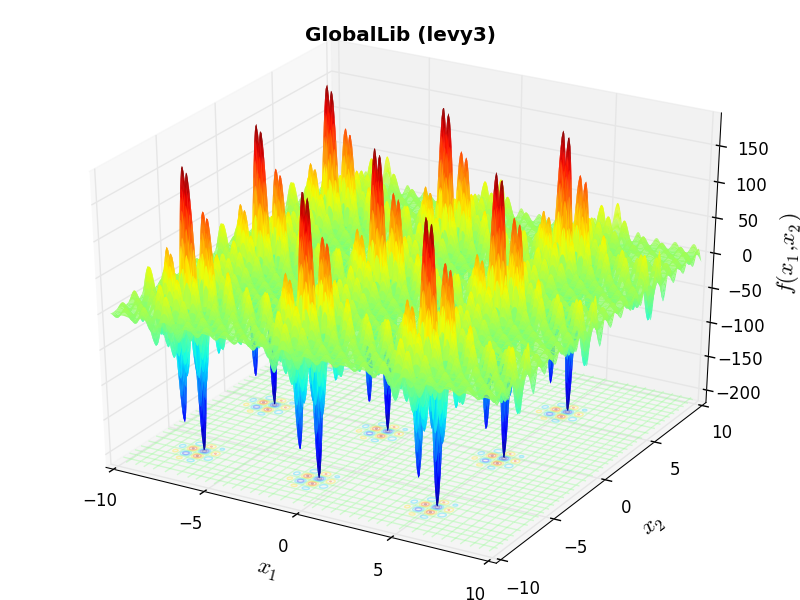
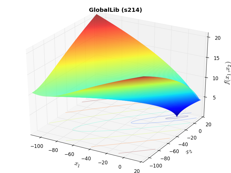
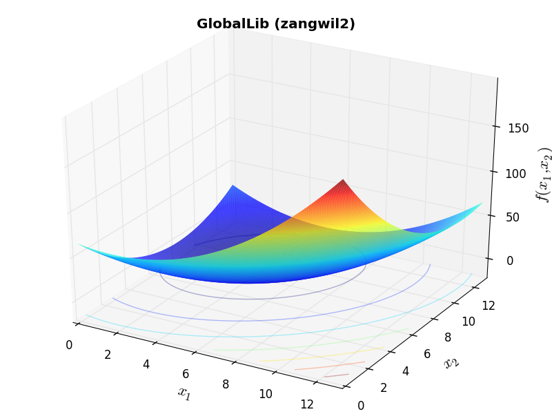
GlobalLib Function levy3	GlobalLib Function s214	GlobalLib Function zangwil2

General Solvers Performances

Table 12.1 below shows the overall success of all Global Optimization algorithms, considering every benchmark function, for a maximum allowable budget of .

The GlobalLib benchmark suite is a relatively easy test suite: the best solver for is MCS, with a success rate of 80.7%, followed at a significant distance by BiteOpt.

Note

The reported number of functions evaluations refers to successful optimizations only.

Table 12.1: Solvers performances on the GlobalLib benchmark suite at NF = 2,000

Optimization Method	Overall Success (%)	Functions Evaluations
AMPGO	60.77%	204
BasinHopping	53.04%	224
BiteOpt	72.38%	495
CMA-ES	43.09%	707
CRS2	43.65%	754
DE	39.78%	935
DIRECT	45.86%	445
DualAnnealing	59.67%	223
LeapFrog	49.17%	439
MCS	80.66%	212
PSWARM	19.34%	1,211
SCE	56.35%	543
SHGO	60.22%	181

These results are also depicted in Figure 12.2, which shows that MCS is the best solver, followed at a significant distance by BiteOpt.

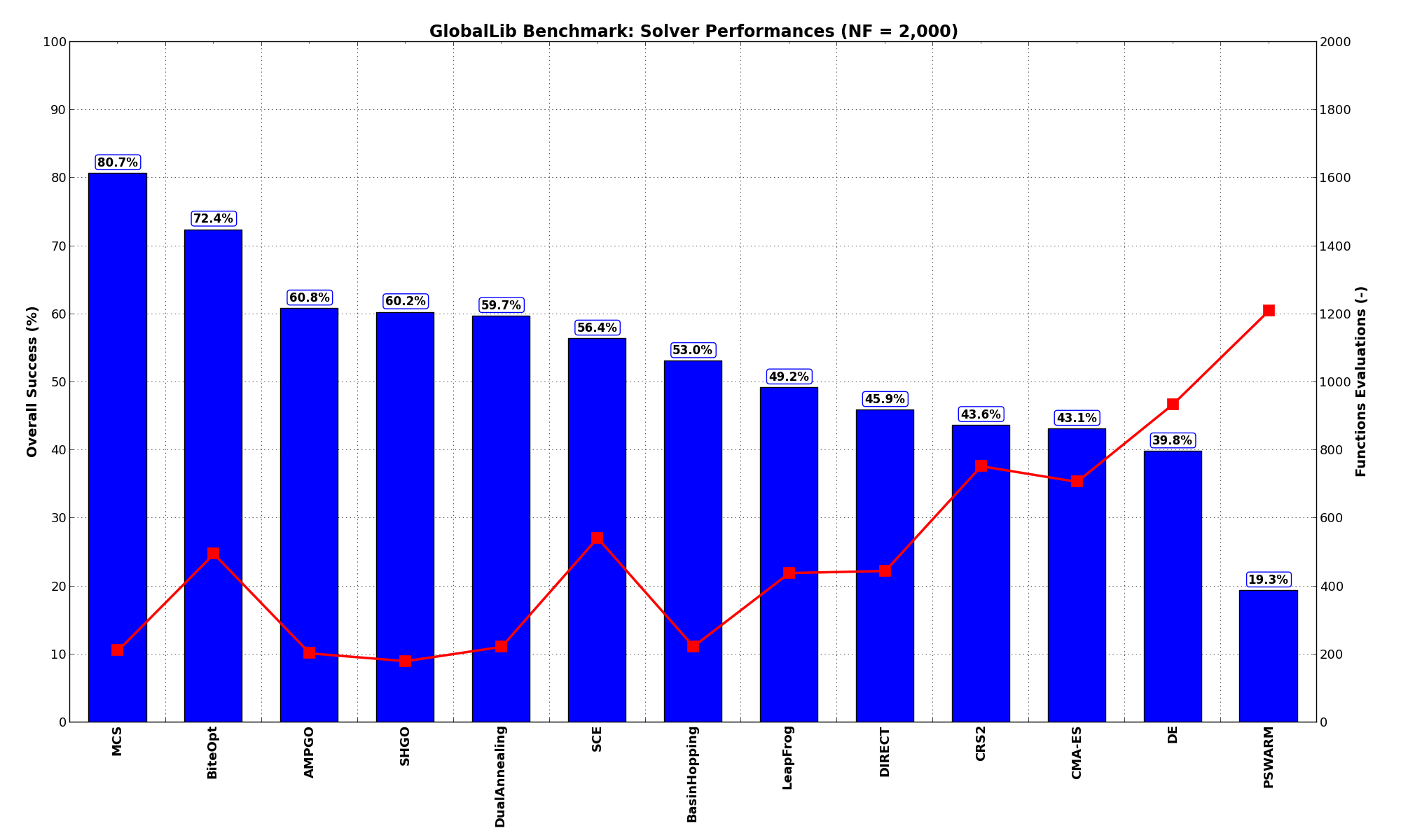
Figure 12.2: Optimization algorithms performances on the GlobalLib test suite at

Pushing the available budget to a very generous , the results show MCS still keeping the lead, with BiteOpt much closer now and AMPGO trailing a bit behind. The results are also shown visually in Figure 12.3.

Table 12.2: Solvers performances on the GlobalLib benchmark suite at NF = 10,000

Optimization Method	Overall Success (%)	Functions Evaluations
AMPGO	71.82%	892
BasinHopping	53.59%	260
BiteOpt	79.01%	963
CMA-ES	54.14%	1,691
CRS2	67.40%	1,786
DE	65.19%	2,743
DIRECT	48.62%	647
DualAnnealing	62.98%	416
LeapFrog	54.70%	817
MCS	85.08%	518
PSWARM	44.75%	2,542
SCE	66.30%	1,189
SHGO	61.88%	299

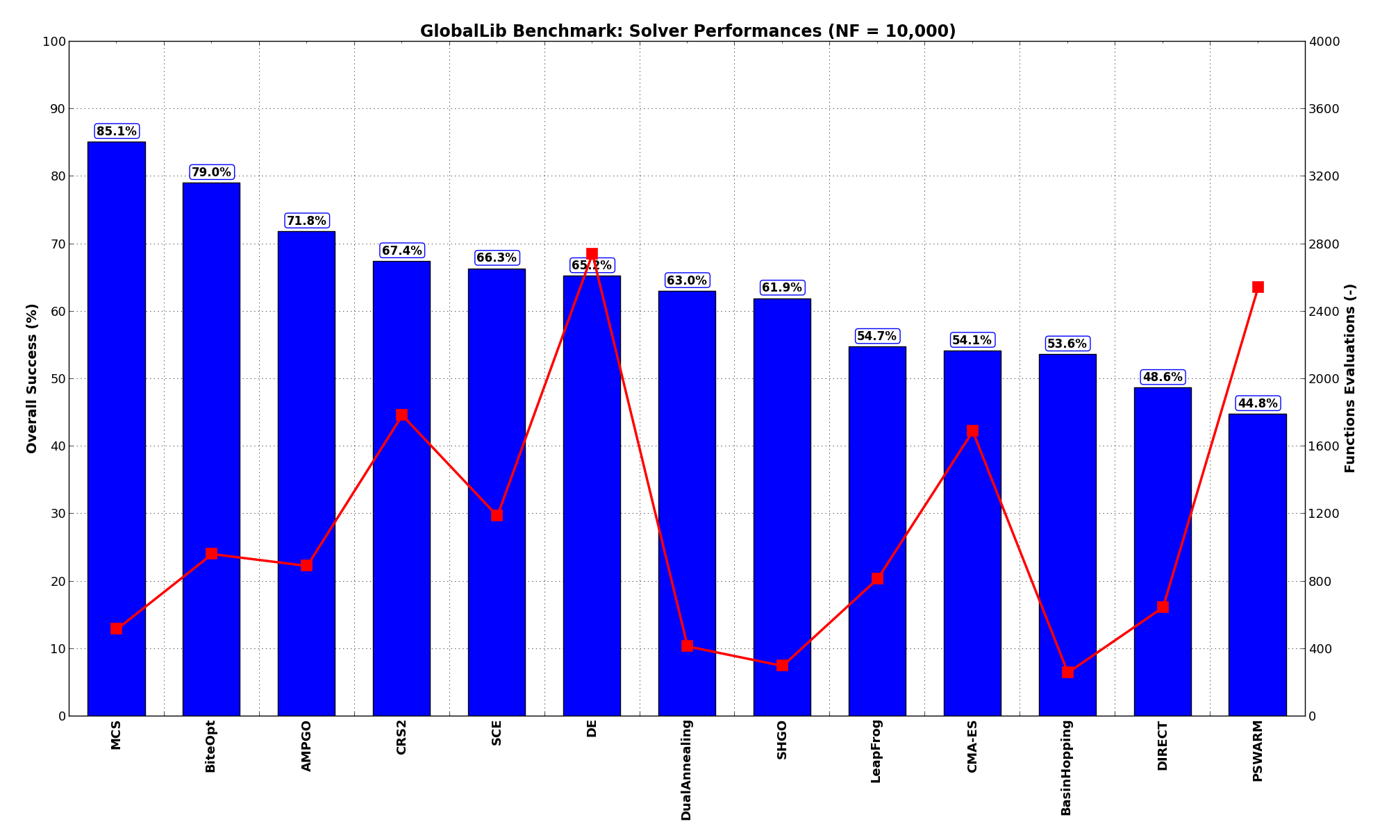
Figure 12.3: Optimization algorithms performances on the GlobalLib test suite at

Sensitivities on Functions Evaluations Budget

It is also interesting to analyze the success of an optimization algorithm based on the fraction (or percentage) of problems solved given a fixed number of allowed function evaluations, let’s say 100, 200, 300,... 2000, 5000, 10000.

In order to do that, we can present the results using two different types of visualizations. The first one is some sort of “small multiples” in which each solver gets an individual subplot showing the improvement in the number of solved problems as a function of the available number of function evaluations - on top of a background set of grey, semi-transparent lines showing all the other solvers performances.

This visual gives an indication of how good/bad is a solver compared to all the others as function of the budget available. Results are shown in Figure 12.4.

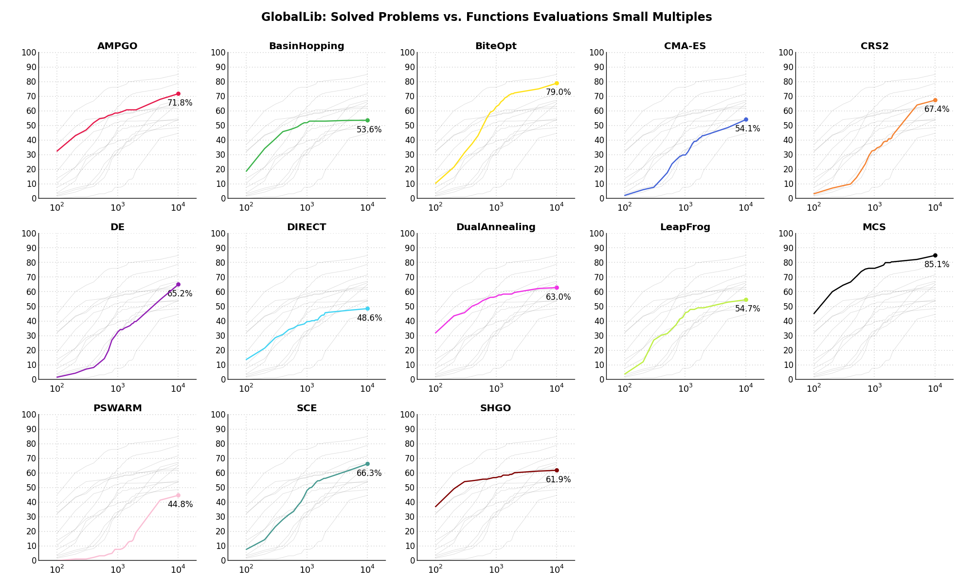
Figure 12.4: Percentage of problems solved given a fixed number of function evaluations on the GlobalLib test suite

The second type of visualization is sometimes referred as “Slopegraph” and there are many variants on the plot layout and appearance that we can implement. The version shown in Figure 12.5 aggregates all the solvers together, so it is easier to spot when a solver overtakes another or the overall performance of an algorithm while the available budget of function evaluations changes.

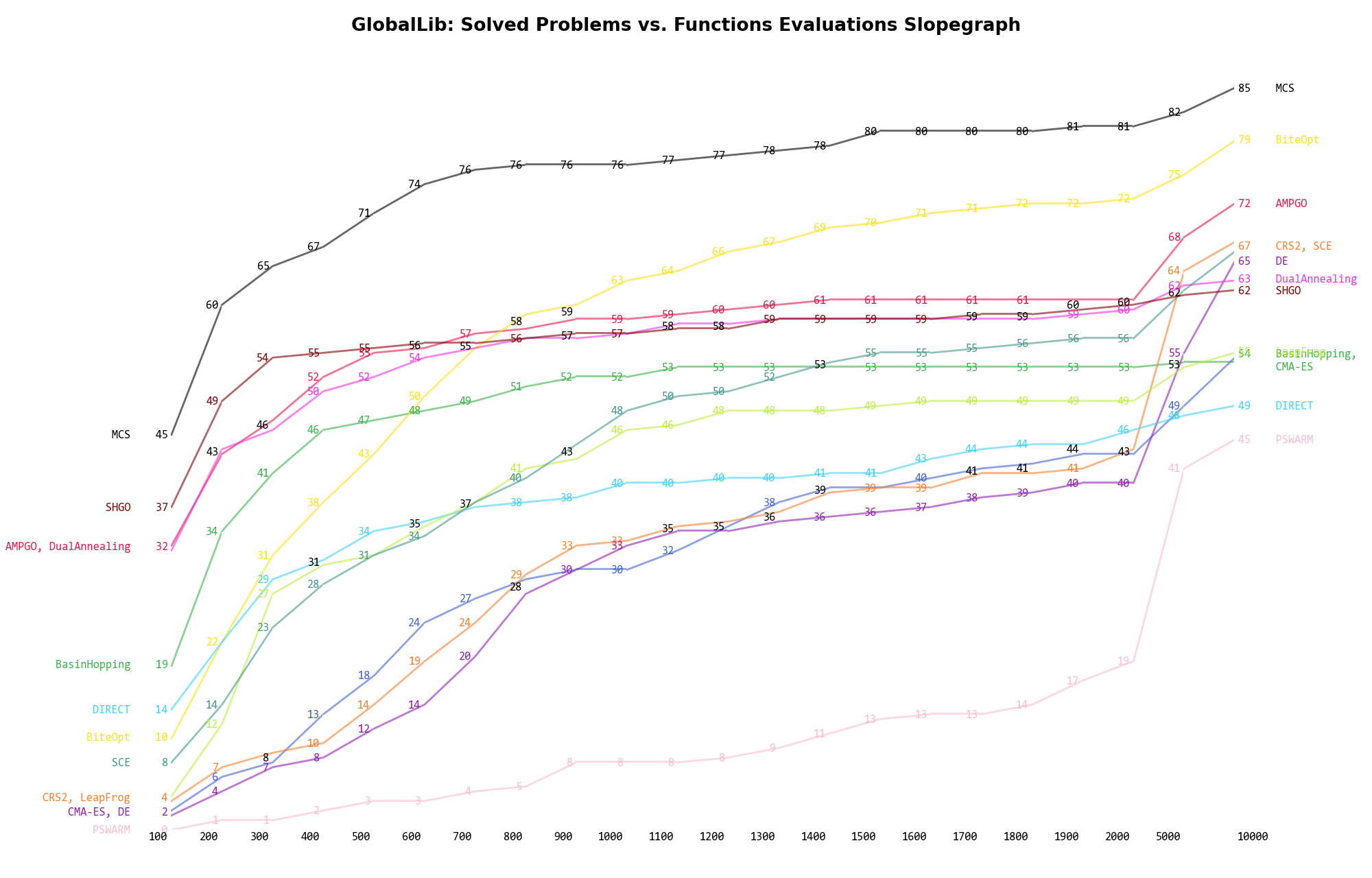
Figure 12.5: Percentage of problems solved given a fixed number of function evaluations on the GlobalLib test suite

A few obvious conclusions we can draw from these pictures are:

1. For this specific benchmark test suite, no matter your function evaluations budgets, MCS is always going to be the best choice among solvers.
2. Starting from around 800 function evaluations, BiteOpt overtakes all other solvers to position itself in second place.
3. For very large allowances in terms of functions evaluations, then BiteOpt and AMPGO become competitive, while still trailing behind MCS.